

Appendix: Mathematical Background#
The models and selection criteria used throughout the tutorial draw on the general log-contrast and perspective-estimation framework of [C1, M9], the tree-aggregation model of [C4], and the latent (sparse + low-rank) graphical model of [M6, M7].
Notation#
Let \(X \in \mathbb{R}^{n \times p}\) be the transformed abundance matrix for \(n\) samples and \(p\) features (ASVs). The centered log-ratio (clr) and modified clr (mclr) transforms map compositional counts into Euclidean space [M5]. For the 300-ASV Atacama table \(n = 54\) and \(p = 300\). \(S\) denotes the empirical covariance (or correlation) matrix of \(X\), and \(\hat{\Theta}\) an estimated precision (inverse covariance) matrix.
Log-contrast regression#
For a continuous outcome \(y \in \mathbb{R}^n\), the sparse log-contrast model [C2, C3, C7] is
where the zero-sum constraint \(\mathbf{1}_p^\top \beta = 0\) makes the fit invariant to the compositional scale.
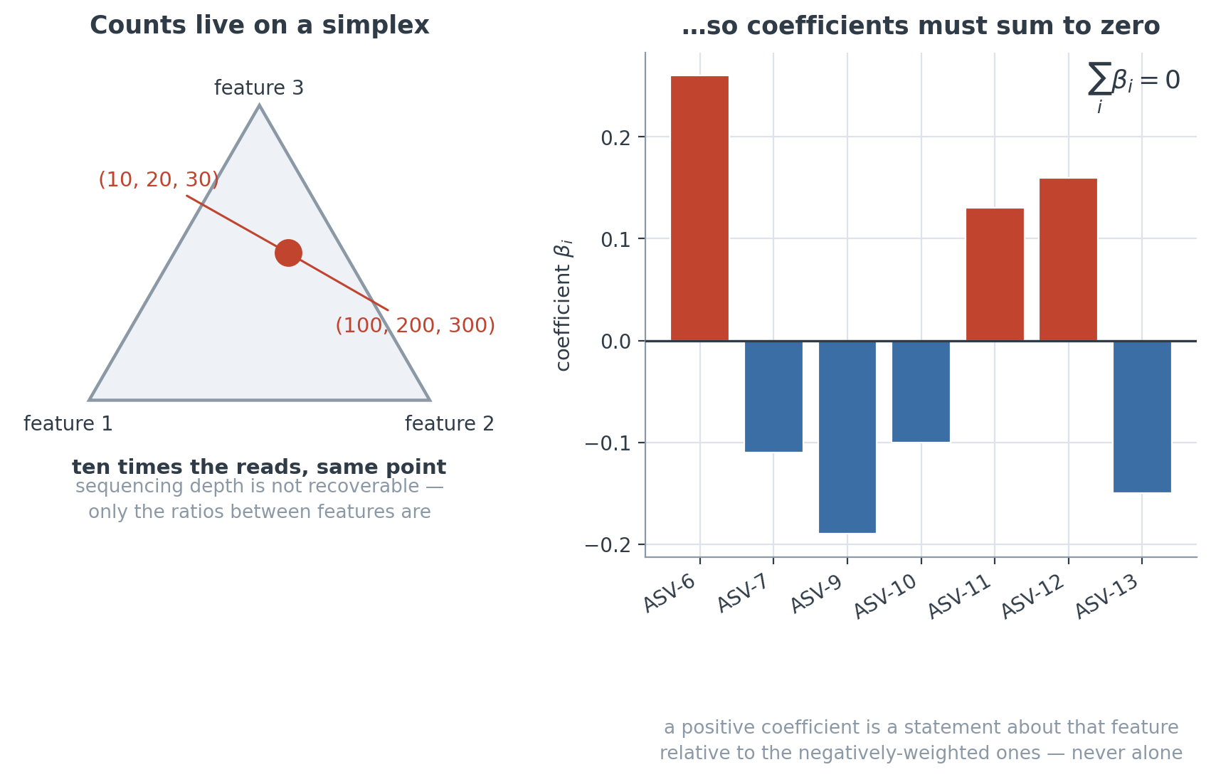
Fig. 27 Scale invariance and the zero-sum constraint. Left: a count vector and any rescaling of it — \((10, 20, 30)\) and \((100, 200, 300)\) — are the same point of the simplex, so sequencing depth is not recoverable from the data and only ratios between features carry information. Right: requiring \(\sum_i \beta_i = 0\) makes the fit depend on those ratios alone. A coefficient is therefore a statement about one feature relative to the negatively-weighted ones, and cannot be read on its own.#
The constraint is not a regularisation choice: it is what makes the model well-posed. Without it, adding a constant to every \(\beta_i\) would change the prediction whenever the total count changes, so the fit would depend on sequencing depth — an artefact of the run rather than of the biology. The loss \(f\) selects the c-lasso formulation:
R1 — standard (least squares): \(f = \lVert y - X\beta \rVert_2^2\), with \(\sigma\) fixed.
R2 — Huber: \(f = h_\rho(y - X\beta)\), robust to outliers.
R3 — concomitant (least squares): \(\ \lVert y - X\beta \rVert_2^2 / (2\sigma) + (n/2)\,\sigma\), jointly estimating \(\sigma\).
R4 — concomitant Huber: the robust analogue, with the linear term \(n\,\sigma\).
The concomitant formulations R3/R4 estimate the noise level \(\sigma\) jointly with \(\beta\) and have no tuning parameter for \(\sigma\): the coefficients \(n/2\) (R3) and \(n\) (R4) are fixed constants that fall out of the perspective function of the respective loss [M9, M10], not hyperparameters.
trac: tree-aggregation#
The trac model [C4] reparameterizes the log-contrast problem on the taxonomic tree. With \(A\) the binary ancestor matrix mapping the \(p\) leaves to their \(t\) tree nodes, the solver fits node coefficients \(\gamma\) with \(\beta = A\gamma\) under a weighted \(\ell_1\) penalty \(\lVert w \odot \gamma \rVert_1\), so that selection acts on internal nodes (aggregated clades) rather than individual ASVs — “tree-aggregation of compositional data”.
Graphical lasso#
The graphical lasso [M1, M11] estimates microbial association networks,
where \(\lVert \cdot \rVert_{1,\text{od}}\) is the off-diagonal \(\ell_1\) penalty and edges correspond to nonzero off-diagonal entries of \(\hat{\Theta}\).
Latent variables: sparse + low-rank (SLR)#
Unobserved environmental/technical factors induce dense confounding. The latent-variable graphical model [M6, M7] decomposes the precision as a sparse part \(\hat{\Theta}_S\) minus a low-rank part \(\hat{L}\),
with \(\lVert \cdot \rVert_\star\) the nuclear norm. The sparse part carries the direct microbial interactions. The rank of \(\hat{L}\) counts the latent factors, and a larger \(\mu\) shrinks that rank. Robust PCA can recover the low-rank subspace [M8].
Model selection#
eBIC for the single graphical lasso#
Along a path of \(\lambda\) values the solver scores each fitted \(\hat{\Theta}\) with the extended BIC [M2]:
where \(|E| = \tfrac{1}{2}\big(\#\{\hat{\Theta}_{ij} \neq 0\} - p\big)\) is the number of off-diagonal edges and \(\gamma \in [0,1]\) tunes the extra edge penalty. \(\gamma = 0.5\) is the conventional choice. The Atacama chapters use \(\gamma = 0.3\), which selects \(\lambda = 0.8\) for the 300-ASV network.
Cross-validation for log-contrast regression#
Log-contrast models are selected by \(k\)-fold cross-validation with the one-standard-error rule, or alternatively by stability selection [M4] or a theoretically-derived fixed penalty [C7]. The reported out-of-sample \(R^2\) is the average over the folds.
Comparing the latent subspace and the regression coefficients#
Two quantities relate the graphical model’s latent structure to the regression tasks, with \(\hat{L} = U\Lambda U^\top\) truncated to the top two eigenvectors, giving loadings \(\ell_j = u_j / \sqrt{\lambda_j}\):
Robust-PC / covariate association \(m_t = \max_j \lvert \operatorname{cor}(z_j, y^{(t)}) \rvert\), the strongest correlation of any robust principal component \(z_j\) with task \(t\)’s outcome.
Rank-2 subspace energy \(q_t = \lVert U^\top \hat{\beta}^{(t)} \rVert_2^2 / \lVert \hat{\beta}^{(t)} \rVert_2^2\), the fraction of the log-contrast coefficient vector lying in the latent subspace, with a permutation \(p\)-value.
Across tasks, \(m_t\) and \(q_t\) are strongly rank-correlated (Spearman \(\rho = 0.90\)), which is the quantitative basis for choosing rank 2.
All references are collected on the References page.