

Predict & Summarize#
regress and classify produce a CLASSOProblem artifact, which is a zarr
archive — not something you can read. Two actions turn it into something you can:
qiime classo predict applies the fitted coefficients to a table the model has
never seen, and qiime classo summarize renders everything as a browsable
visualization.
Run them in that order. summarize accepts predictions as an optional input and
adds a held-out-performance panel to every model-selection tab when you supply
them; without them you get the fit and nothing about generalization.
The commands below run on the log-contrast regression artifacts built in
Log-Contrast Regression —
data/regresstaxa_lc.qza for the model, data/regress-xtest_lc.qza for the
held-out table — and on the trac artifacts from
Log-Contrast Regression with trac where a taxonomy is
needed.
Run them from the tutorial root ~/q2-hdstats-tutorial — the directory that
contains data/ — and not from the smoke-test/ directory used in
Synthetic Data with Known Truth.
Predicting on a held-out table#
qiime classo predict \
    --i-features data/regress-xtest_lc.qza \
    --i-problem data/regresstaxa_lc.qza \
    --o-predictions data/regress-predictions_lc.qza
predict takes no parameters. Everything it needs — which model-selection
blocks were run, which coefficient vectors to apply — is read from the problem
artifact, and it produces one prediction vector for each block that was enabled
at fit time:
Block enabled at fit |
Predictions produced |
|---|---|
|
one vector per λ on the path |
|
one vector, from the CV refit coefficients |
|
one vector, from the stability-selection refit coefficients |
|
two vectors, before and after refit |
Important
The prediction table must contain every column the model was trained on, by
name. predict does not align tables positionally; it walks the model’s stored
label vector and pulls each column out of your table by name. A missing or
renamed column is a hard failure, not a silently dropped feature.
The held-out table therefore has to come from the same feature table as the
training table — which is exactly what qiime sample-classifier split-table
gives you, since it splits rows and leaves columns untouched. Do not hand
predict a table you built with a separate add-covariates call: the one-hot
expansion of a categorical covariate names its columns after the values it
happens to observe, so a different subset of samples can yield a different set
of columns.
The intercept entry is handled specially: it is not looked up in your table,
it is filled with ones. So a model fitted with the default --p-intercept needs
no intercept column in the prediction table, and adding one would be ignored.
Note
predict emits an artifact of type CLASSOProblem — the same type as the
output of regress. It does not contain a problem, it contains predictions, and
the two are not interchangeable. Because the types match, QIIME 2 accepts a
predictions artifact for summarize --i-problem, or a problem artifact for
summarize --i-predictions, and the failure surfaces as a confusing key error
deep inside the visualizer. Keep the two apart by filename.
Summarizing without a taxonomy#
qiime classo summarize \
    --i-problem data/regresstaxa_lc.qza \
    --i-predictions data/regress-predictions_lc.qza \
    --p-maxplot 200 \
    --o-visualization data/regresstaxa_lc.qzv
--i-taxa is optional. Omitting it costs you exactly two panels — the taxonomic
tree on the Overview tab and the selected-nodes tree on the Stability Selection
tab. Everything else, including all coefficient tables, plots and CSV exports, is
identical.
Summarizing with a taxonomy#
qiime classo summarize \
    --i-problem data/regresstaxa_trac.qza \
    --i-taxa data/classification.qza \
    --i-predictions data/regress-predictions_trac.qza \
    --p-maxplot 200 \
    --o-visualization data/regresstaxa_trac.qzv
Supplying --i-taxa adds tree.html to the Overview tab and stabsel-tree.html
to the Stability Selection tab, the latter with the selected nodes highlighted
against the unselected ones.
The tree is built by pruning the taxonomy down to the nodes whose names appear in
the model’s label vector. That is why the panel is worth having on a trac model,
whose labels are internal taxonomic nodes produced by
qiime classo add-taxa: the plot then shows you where in the hierarchy the
selected aggregates sit. On a plain log-contrast model the labels are tips
(individual ASV IDs) plus covariate column names, so the pruned tree collapses to
a root with its tips and tells you very little.
Covariate columns added by add-covariates are never in the taxonomy. They are
absent from the tree panel, which is expected and is not an error.
Note
Pass the same taxonomy artifact you used to build the model. A taxonomy whose tip names do not match the model’s labels produces a tree with nothing on it, without complaining.
--p-maxplot, and what it truncates#
--p-maxplot defaults to 200 and caps how many bars are drawn in the
coefficient and stability plots. It is a plotting parameter only: nothing errors,
nothing is logged, and no exported data is affected.
It governs two rules.
Coefficient bar plots (cv-refit.html, stabsel-refit.html,
lam-beta.html, lam-refit.html). Zero coefficients are always dropped. If the
number of non-zero coefficients still exceeds --p-maxplot, only the
maxplot largest in absolute value are kept. For a sparse fit this cap almost
never binds — a lasso solution with more than 200 non-zero entries is not a
sparse solution.
The stability-selection profile (stabsel-graph.html). This plot is
different: it shows every coefficient, selected or not, because the point of
the profile is to see the whole distribution of selection probabilities against
the threshold line. The cap is therefore compared against the total number of
coefficients, and if that total exceeds --p-maxplot the plot keeps only the
maxplot features with the highest selection probability.
Set --p-maxplot to at least the number of design columns, which is the number
of features in the model plus one for the intercept. Below that value the profile
silently loses its low-probability tail. The selected features survive — they are
the highest-probability ones by construction — but the threshold line no longer
has anything to separate them from, the bar index on the x-axis stops
corresponding to feature position, and a truncated profile looks exactly like a
genuinely concentrated one.
You do not have to guess the number. Build the .qzv once, read Number of
features off the Overview tab, add one for the intercept, and rebuild with
--p-maxplot at least that large. On a Tier-1 problem the default 200 is
comfortably above it; on the 300-ASV problem of
Log-Contrast Models at Scale it is not.
Note
Raising --p-maxplot past a few hundred makes the plots slow to render and hard
to read — every bar becomes a sliver. If the full profile is genuinely too wide
to plot, work from StabSel-prob.csv instead, which is complete regardless of
--p-maxplot.
The complete, untruncated results are always available from the visualization regardless of this parameter:
File |
Contents |
|---|---|
|
the design matrix as fitted |
|
the response vector |
|
the constraint matrix |
|
β at every λ on the path |
|
the CV refit coefficients |
|
selection probability for every feature |
|
the fixed-λ refit coefficients |
The HTML tables of selected parameters on the CV, Stability Selection and LAM
fixed tabs are also unaffected by --p-maxplot.
The six pages#
summarize renders six templates: index.html, which is the tab shell that
wraps everything, plus one page each for overview, path, cv,
stabsel and lam-fixed. All six are rendered on every run, but a tab only
appears in the navigation if the corresponding block was enabled at fit time —
so a model fitted with --p-no-stabsel produces a .qzv with no Stability
Selection tab. Overview is always present.
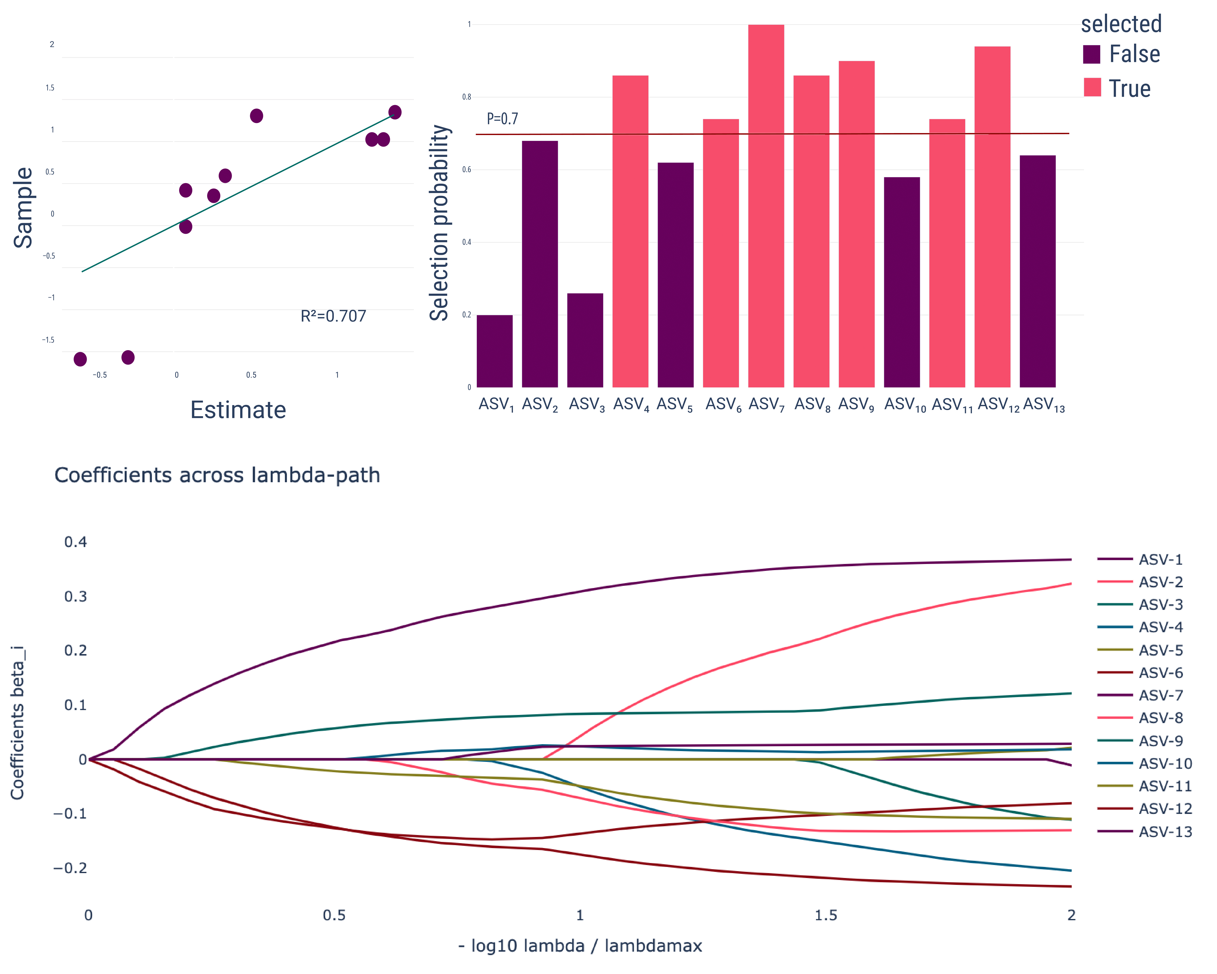
Fig. 14 Three of those pages at full size, from a regression on the 13-ASV toy data. Top left is the held-out fit that the performance table summarises; top right is Stability Selection, one bar per feature against the threshold; and bottom is Lambda-path, every coefficient as the penalty relaxes. The x-axis there is \(-\log_{10}(\lambda/\lambda_{\max})\), so the penalty decreases to the right and coefficients leave zero as you move right.#
Log-Contrast Regression shows the same run as a four-panel composite that also includes the Cross-Validation page. Use the composite for an overview and the figure above when you need to identify individual features.
Overview#
The problem as the solver saw it: total number of samples, number of samples in
the training set, number of features, number of constraints. Then the
formulation, named and rendered as a formula image — R1 through R4 for
regression, C1 or C2 for classification, with ρ shown when the Huber loss is
in play. The three CSV downloads for the design, response and constraint
matrices. Finally the taxonomic tree, if --i-taxa was given.
The sample counts are the first thing to check: Number of samples in total
counts every sample with a non-missing response in the metadata column, while
Number of samples in the training set counts the rows that survived the join
with your feature table. A gap between them means samples were dropped, and
regress --verbose prints which ones.
Lambda-path#
Requires --p-path. Reports the numerical method, the smallest λ and the number
of grid points, and the solve time. The main panel is the coefficient trajectory
against −log₁₀(λ/λ_max), with a path.csv download. Coefficients that never rise
above a small fraction of the largest coefficient anywhere on the path are left
out of the plot to keep it legible.
If the model was fitted with --p-concomitant, a second panel plots the
estimated scale σ along the same axis — a useful diagnostic in its own right,
since σ should decline and then flatten as the model saturates.
If predictions were supplied, a third panel plots held-out error against λ.
Note
The path prediction panel only uses samples that are in the prediction table
and were not in the training set. Predict on the training table and that set
is empty, which does not raise — it produces a flat, meaningless error curve.
Always point predict at a held-out table.
Cross-Validation#
Requires --p-cv. Reports the numerical method, number of subsets, whether the
one-standard-error rule was used, the λ grid, and the seed. Both lambda_1SE and
lambda_min are shown, as fractions of λ_max, regardless of which one the refit
used.
Then the table of selected parameters with their refit coefficients, the
CV-beta.csv download, a bar plot of those coefficients, and the cross-validation
curve itself: mean error against −log₁₀(λ/λ_max) with error bars, and vertical
lines at lambda_min and lambda_1SE. The y-axis is mean squared error for
regression and misclassification rate for classification.
With predictions supplied, a performance table and an observed-versus-predicted scatter are added. The scatter colours points by training membership and draws the identity line.
Stability Selection#
Requires --p-stabsel. Reports the full parameter block — method, true_lam,
the theoretical λ, the λ actually used, lamin, B, q, percent_nS, the
threshold and the seed — followed by the solve time and the number of selected
parameters.
The core of the page is the stability profile: a table of the selected features
with their probabilities, the StabSel-prob.csv download, and the bar plot of
selection probability for every feature with the threshold drawn across it,
selected bars coloured differently from unselected ones. Below that, the refit
coefficients on the selected support, then the prediction panels, then the
taxonomic tree with the selected nodes highlighted if --i-taxa was given.
Note
Known gap: the stability profile across the λ-path never renders. The
template has a panel for it, and the underlying data exists for
--p-stabsel-method first, but the flag that controls the panel is
unconditionally forced off in the visualizer. You get the profile at the selected
λ, not its evolution along the path. Nothing errors; the panel is absent.
LAM fixed#
Requires --p-lamfixed. Reports the numerical method, whether λ was given as a
true λ or as a fraction of λ_max, λ_max itself and the theoretical λ; then the
solve time, the λ actually used, and the estimated σ.
Two coefficient plots: the refit coefficients, re-estimated on the selected support without the penalty, and the pre-refit penalized coefficients. Quote the refit values as effect sizes; read the pre-refit values to see how hard the penalty is biting. With predictions supplied you get a prediction panel for each.
Reading the performance table#
The prediction table that appears on the CV, Stability Selection and LAM fixed
tabs has six rows, and only some of them apply to your problem. The ones that do
not are filled with the literal string inappropriate rather than being hidden:
a regression fit shows inappropriate for positives, negatives, false positives
and false negatives, and a classification fit shows inappropriate for R². That
is expected output, not a bug.
Important
The value labelled R square is the squared Pearson correlation between observed and predicted values, not the fraction of variance explained. The two coincide only for an unbiased, correctly scaled predictor. A shrunken lasso fit is neither, so the reported number is systematically the more flattering of the two: it is invariant to any linear rescaling of the predictions, and it will not notice that your model is uniformly biased. Read it as a measure of rank agreement, and read the observed-versus-predicted scatter against the identity line to see whether the calibration is there.
The Number of sample row counts the samples common to the prediction table and the response column. Predict on a held-out table and it is your test-set size; predict on the full table and it silently becomes an in-sample number.
Known failure modes#
--i-problemand--i-predictionshave the same semantic type. Swapping them type-checks and then fails inside the visualizer.Predicting on the training table produces an in-sample R² and a degenerate λ-path error curve. Neither is flagged.
--p-maxplotbelow the number of design columns silently truncates the stability profile.A taxonomy that does not match the model labels produces an empty tree panel rather than an error.
Every plot pane blank? That was a real defect in older q2-classo, where the plot-writing calls were commented out while the templates still referenced the iframes. It is fixed in current builds — see Troubleshooting.
Note
No R² values, sample counts, selected supports or runtimes are quoted here, because none of these commands has been re-run. The description of each page comes from the templates and the visualizer code; the numbers they will show are yours to generate.
Next#
Interpretation — what a selected support and a set of log-contrast coefficients actually mean.
Advanced: Choosing a Model — if the tabs disagree with each other.
Log-Contrast Models at Scale — the same two actions where
--p-maxplotstarts to matter.