High-Dimensional Example: q2-classo on 300 Atacama ASVs

q2-classo fits one cross-validated log-contrast regression per continuous environmental covariate, predicting it from the microbiome on the same 300-ASV, 54-sample Atacama design used in the high-dimensional graphical-lasso chapter. The fits reproduce the reference analysis of Christian L. Müller.

Important

Build the design with qiime classo transform-features, not with qiime gglasso transform-features.

The gglasso action is no longer broken. Keep the two chains independent and a change on the network side cannot quietly alter the regression results. classo’s own transform also takes the raw counts directly, which is the shorter path.

Both are now valid inputs. Until QIIME 2 2026.7, only one was: gglasso transform-features stored its output with the axes swapped, so the table’s “samples” were feature IDs, regress found no overlap with the outcome on the sample index, and c-lasso failed deep inside with

IndexError: index 0 is out of bounds for axis 0 with size 0

on a design of shape (0, 54). If you hit that on an older artifact, that is the cause. Regenerate the artifact rather than transposing it by hand: calculate-covariance was compensating for the same swap, and the two give the right answer only together. See Troubleshooting.

Setup

Each of the 15 continuous covariates serves once as the outcome; missing outcome values are mean-imputed. Every model uses the log-contrast formulation with an intercept and is selected by 5-fold cross-validation under the one-standard-error rule along a log-spaced \(\lambda\) path.

Build the design once:

qiime classo transform-features \
    --i-features data/atacama-top-300-table.qza \
    --o-x data/atacama-top-300-classo-clr.qza

Then fit one model per outcome:

qiime classo regress \
    --i-features data/atacama-top-300-classo-clr.qza \
    --m-y-file data/atacama-classo-outcomes-mean-imputed.tsv \
    --m-y-column "<outcome>" \
    --p-concomitant \
    --p-path --p-path-nlam-log 60 --p-path-lamin-log 0.001 \
    --p-cv --p-cv-subsets 5 --p-cv-seed 1 --p-cv-one-se \
    --p-cv-nlam 60 --p-cv-lamin 0.001 --p-cv-logscale \
    --p-no-stabsel --p-no-lamfixed \
    --o-result "<outcome>-cv5.qza"

--p-cv-nlam takes a single dash before nlam. The old --p-cv--nlam spelling still works but is deprecated.

Recomputed fits

All 15 fits were re-run on QIIME 2 2026.7. slurm/12_classo_summary.sh generates the table below from the solution artifacts:

Table 3 Cross-validated log-contrast fits, 300 ASVs x 54 samples

outcome	selected features	lambda (min CV)	CV error (min)	max |beta|
amplicon-concentration	12	0.31012	22.643	10.4
average-soil-relative-humidity	8	0.27585	391.74	74.23
average-soil-temperature	5	0.39194	16.025	15.87
depth	1	0.62605	0.21301	1.981
ec	1	0.49535	0.33565	0.3763
elevation	5	0.39194	4.9722e+05	2985
extract-concen	33	0.24538	14.591	4.017
percent-relative-humidity-soil-100	13	0.19415	591.74	50.79
percentcover	22	0.27585	7.1704	2.018
ph	16	0.21826	0.37138	7.868
relative-humidity-soil-high	5	0.13664	307.46	88.45
relative-humidity-soil-low	8	0.44062	650.3	53.58
temperature-soil-high	7	0.34864	9.0494	22.93
temperature-soil-low	4	0.55688	20.133	7.683
toc	1	0.39194	3.4997e+06	1068

Read the sparsity, not the error scale: the CV error is in the outcome’s own units squared, so it is comparable across \(\lambda\) for one outcome and not across outcomes. The comparable quantity is how many of the 300 ASVs survive — from a single feature for depth, ec and toc up to thirty-three for extract-concen.

Prediction from ASVs only (base R1)

Important

The \(R^2\) table below has NOT been reproduced. The recompute reports cross-validated error, which is what the solution artifact stores. Turning that into an out-of-sample \(R^2\) needs a qiime classo predict pass on held-out samples, and that pass has not been run. The figures below are carried over from the reference analysis and are retained for their ranking of the outcomes. Treat them as unverified and do not quote an individual value.

The same applies to the joint and filtered \(R^2\) values further down, and to the named first-selected taxon.

The out-of-sample \(R^2\) (mean across the 5 folds) shows which environmental variables are predictable from the 300 ASVs alone:

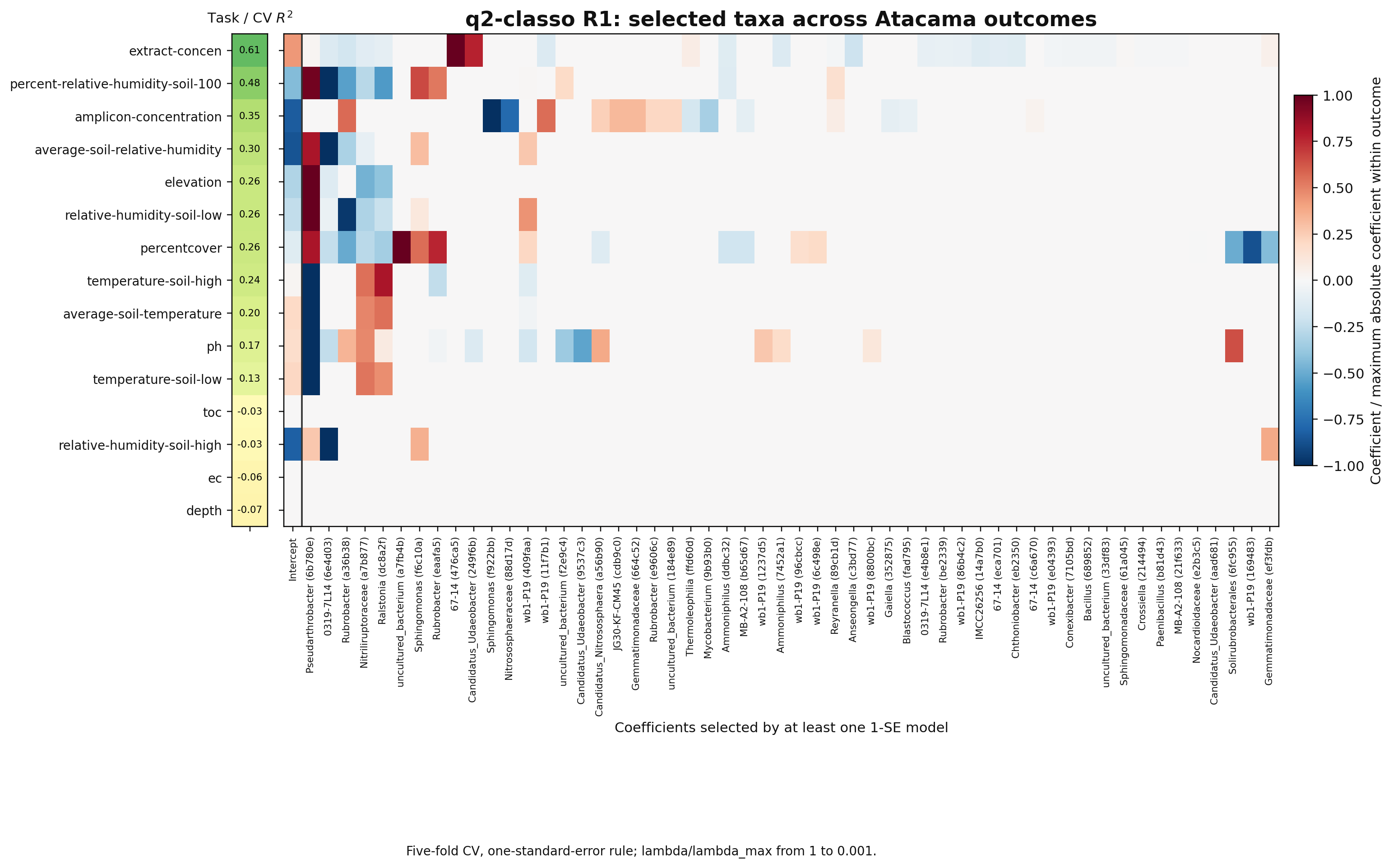
Fig. 20 One row per outcome, ordered by cross-validated \(R^2\) (left column); one column per ASV selected by at least one 1-SE model. Colour is the coefficient divided by the largest absolute coefficient within that row, so shades are comparable along a row and not down a column.

Most outcomes are not predictable from the microbiome alone: only the top two clear \(R^2 = 0.4\). The bottom four rows (toc, relative-humidity-soil-high, ec, depth) have negative \(R^2\) — the model does worse than predicting the mean, and their rows are correspondingly almost empty. A negative \(R^2\) here is the honest answer rather than a bug. Pseudarthrobacter (6b780e) is the most widely shared predictor, carrying weight in nearly every outcome that is predictable at all — the genus discussed in Network interpretation.

Important

The ph row is contaminated. Eight samples in the Atacama metadata carry ph = 0, a missing-value sentinel rather than a measurement — pH 0 is not a soil. Those rows enter the regression as genuine values sitting about 2.8 standard deviations below the mean. Do not interpret the ph result in this figure or in the next one. See q2-classo parameters for the check that surfaces it.

Outcome	CV \(R^2\)
extract-concen	0.61
percent-relative-humidity-soil-100	0.48
amplicon-concentration	0.35
average-soil-relative-humidity	0.30
elevation	0.26
relative-humidity-soil-low	0.26
percentcover	0.26
temperature-soil-high	0.24
average-soil-temperature	0.20
ph	0.17
temperature-soil-low	0.13
toc / relative-humidity-soil-high / ec / depth	\(\le 0\)

The first selected taxon (largest-magnitude coefficient column, after the intercept) is a Pseudarthrobacter ASV — a genus characteristic of the Atacama soil community (see the interpretation notes).

Adjusting for environmental covariates (joint and filtered)

Two variants add the other covariates as extra predictors (each rescaled and L2-normalized, covariate penalty weight 0.1626):

• Joint — add every other covariate as a predictor.

• Filtered adjustment — add only covariates that are not strongly correlated with the outcome (Pearson \(\lvert r\rvert < 0.80\)), so a covariate that is essentially a proxy for the outcome cannot leak it.

Adding covariates takes two steps. First, build the augmented design from the ASV design plus the chosen covariate(s), which produces new features, constraint and weights artifacts:

qiime classo add-covariates \
    --i-features data/atacama-top-300-classo-clr.qza \
    --m-covariates-file data/atacama-classo-outcomes-mean-imputed.tsv \
    --p-to-add <covariate> --p-rescale --p-w-to-add 0.162565105 \
    --o-new-features <design>.qza --o-new-c <c>.qza --o-new-w <w>.qza

Then run the same cross-validated regression on the augmented design, passing the constraint and weights from the first step:

qiime classo regress \
    --i-features <design>.qza --i-c <c>.qza --i-weights <w>.qza \
    --m-y-file atacama-classo-outcomes-mean-imputed.tsv --m-y-column <outcome> \
    --p-do-yshift --p-path --p-path-nlam-log 120 --p-path-lamin-log 0.0001 \
    --p-cv --p-cv-subsets 5 --p-cv-seed 1 --p-cv-one-se \
    --p-cv-nlam 120 --p-cv-lamin 0.0001 --p-cv-logscale \
    --p-no-stabsel --p-no-lamfixed --p-no-concomitant --p-no-huber --p-intercept \
    --o-result <outcome>-joint-r1-cv5.qza

Adding covariates sharply increases the predictability of the physically coupled variables — soil temperature and humidity among them — but the filtered analysis removes most of that gain, placing its source in the outcome-correlated covariates rather than in the microbiome:

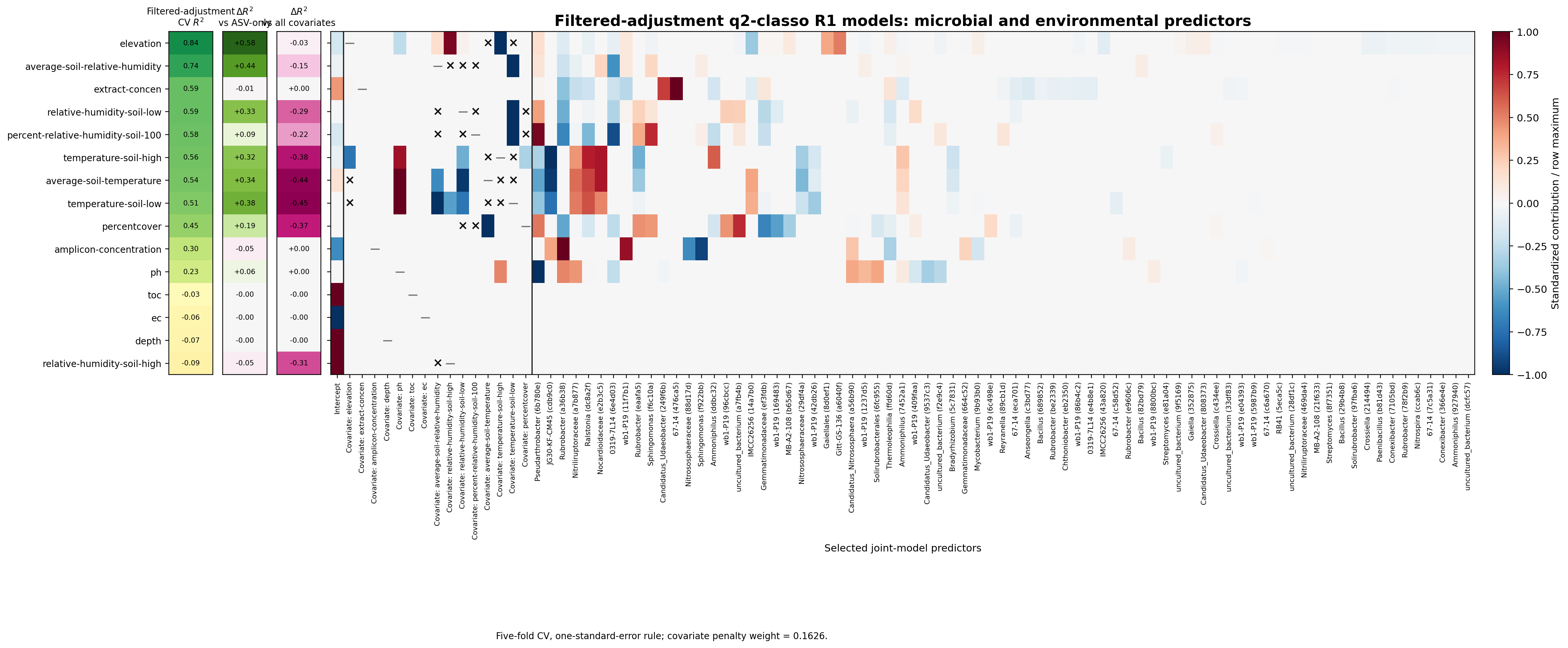
Fig. 21 The filtered-adjustment models. Same layout as Fig. 20, but the predictor block now begins with the added covariates (left of the vertical rule) before the ASVs, and three score columns replace one: the filtered \(R^2\), its gain over the ASV-only model, and its loss relative to using all covariates.

elevation reaches 0.84, of which \(+0.58\) comes from covariates and only \(-0.03\) is given up by filtering — its predictors were never proxies. The soil-temperature outcomes behave the opposite way: temperature-soil-low gains \(+0.38\) over ASVs alone but loses \(-0.45\) against the unfiltered model, so most of that apparent skill was one covariate standing in for the outcome. toc, ec and depth stay negative with \(\Delta R^2 \approx 0\) throughout, and their near-empty rows show the model selecting little beyond the intercept.

Note

The × and − marks in the covariate block have no legend. The figure is carried over from the reference analysis, its marker legend was not preserved with it, and no script in this repository regenerates it. Read the colours and the three labelled score columns, and treat the markers as unexplained rather than inferring a meaning for them.

Outcome	ASV-only	Joint (all cov.)	Filtered (\(\lvert r\rvert<0.8\))
average-soil-temperature	0.20	0.98	0.54
temperature-soil-low	0.13	0.96	0.51
temperature-soil-high	0.24	0.94	0.56
average-soil-relative-humidity	0.30	0.88	0.74
relative-humidity-soil-low	0.26	0.88	0.59
elevation	0.26	0.87	0.84
percentcover	0.26	0.81	0.45
percent-relative-humidity-soil-100	0.48	0.80	0.58
extract-concen	0.61	0.59	0.59

Elevation’s filtered \(R^2\) (0.84) stays close to its joint value (0.87), so its predictability does not depend on outcome-correlated covariates. For the temperature variables the joint gain (≈ 0.94–0.98) collapses under filtering (≈ 0.51–0.56). Filter the covariates separately for each outcome.