

Log-Contrast Models Overview#
Microbiome counts have no absolute scale: a sample sequenced twice as deeply gives twice the counts and exactly the same biology. Log-contrast models are built for that — they work in log-ratios and require the coefficients to sum to zero, so the fit depends on the balance between taxa rather than on any number the sequencing run happened to produce.
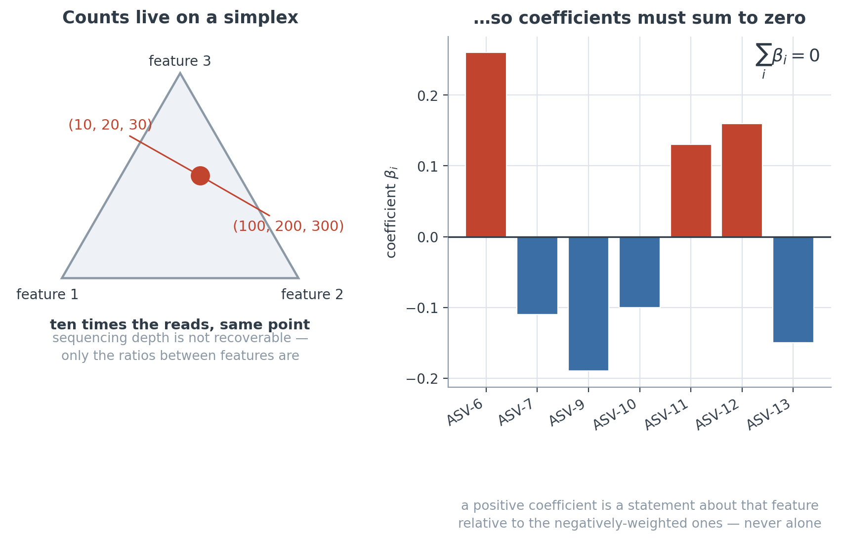
Fig. 10 Scale invariance and the zero-sum constraint. See Appendix: Mathematical Background for the formulation it comes from.#
The formulation#
Relative abundances sum to a constant, so a composition occupies a simplex rather than the whole of Euclidean space. A log-contrast model works around that in three steps:
transform the counts with the centered log-ratio (CLR) or another log-ratio map;
fit a regularized regression or classifier in the transformed space;
read the coefficients as changes in relative abundance.
The same three steps serve a continuous response and a categorical one.
Contents#
1. Data preparation#
Transform a count table to log-ratios, aggregate it on the taxonomy, append environmental covariates, and split it into training and test sets.
2. Regression models#
Predict a continuous outcome (temperature, pH) from community composition:
Log-Contrast Regression: CLR-transformed features, without the taxonomy
trac: aggregates features along the taxonomic hierarchy before selection
3. Classification models#
Predict a categorical outcome such as disease status or habitat type:
Log-Contrast Classification: the same design matrix against a categorical response
trac: identifies predictive taxonomic groups, not only individual features
4. Advanced topics#
Concomitant Formulation: joint estimation of the coefficients and the noise level, for data with heterogeneous variance
5. Interpretation#
What a fitted log-contrast model does and does not say about the community.
Key concepts#
Log-Ratio Transformations: convert compositional data to unrestricted space
CLR (Centered Log-Ratio): the usual choice; centres each sample on its geometric mean
ALR (Additive Log-Ratio): divides by one component taken as the reference
Regularization: prevents overfitting in high-dimensional microbiome data
L1 penalty (Lasso): drives coefficients to exactly zero and so selects a subset of features
Stability selection: keeps the features whose selection probability across subsamples clears a threshold
trac (tree-aggregation of compositional data): uses phylogenetic structure
trac computes adaptive weights from the taxonomic hierarchy
It groups related taxa, so a coefficient attaches to a clade
Prerequisites#
Install the plugins, following Installation.
Read the description of the Atacama dataset.
You will need a working knowledge of regression and classification.
Reading order#
Begin with Data Preparation, then take the branch that matches your response variable:
continuous → Regression
categorical → Classification