Latent Components & Covariates

Choosing the Latent Rank produced a low-rank block \(\hat{L}\) and an integer — its rank — and argued about which integer to keep on parsimony and identifiability grounds, without looking at what the latent dimensions actually are.

qiime gglasso pca projects the samples onto the eigenvectors of \(\hat{L}\) and plots them; Latent-Component PCA covers the mechanics. At rank 2 this table supports a question the 13-ASV example could not: is the latent block modelling the Atacama aridity transect, or is it modelling sequencing depth? A rank-2 subspace has exactly two directions, the study has a small number of plausible global drivers, and there are measured covariates for most of them, so the correspondence is testable.

Note

No figure, correlation or component-to-covariate assignment below has been computed; all of it is pending verification against QIIME 2 2026.7.

Two prerequisites

Both fail unhelpfully:

Important

The solution must come from --p-latent. pca reads solution/lowrank_, which exists only for a latent problem. The SGL solution from Selecting lambda will not work.

--m-sample-metadata-file is effectively required. It is registered as an optional Metadata parameter but is dereferenced unconditionally; omitting it raises an AttributeError on NoneType.

Troubleshooting records both.

--p-n-components must not exceed the achieved rank

pca validates n_components <= rank(L) up front and raises

n_components (N) exceeds the rank of the low-rank component (R).
Pass --p-n-components R or lower.

The pair-plot repeats the check as a defensive assertion, worded n_components (N) is greater than the rank of the low-rank component (R). Requesting exactly as many components as the achieved rank is legitimate — the limit is the rank itself, not one below it:

Solution	\(\mu_1\)	Achieved rank	Largest usable --p-n-components	Pair-plot
atacama-top-300-slr-lambda0.8-rank2.qza	15	2	2	1 panel
atacama-top-300-slr-lambda0.8-mu10.qza	10	5	5	up to 10 panels
atacama-top-300-slr-lambda0.8-mu7.5.qza	7.5	10	10	up to 45 panels

Note

These ranks are measured, not targets: each was read out of the fitted solution, and they are the values the generated map in Choosing the Latent Rank reports.

Note

Read the achieved rank out of your own solution before choosing --p-n-components, rather than copying the table: a different \(\lambda\), a different covariance matrix, or a different GGLasso build can all shift it. If the rank came back lower than expected, the command fails on the guard rather than on anything you can see in the CLI. Leave yourself a margin rather than sizing exactly to a reported rank: the guard uses np.linalg.matrix_rank, whose default tolerance is far finer than the 1e-9 eigenvalue cut the projection itself applies, so it can admit a value for which fewer components actually materialize.

The canonical rank-2 model is the thin case. Rank 2 admits at most --p-n-components 2, which fills exactly one panel of the pair-plot grid — PC1 against PC2, the same scatter the Single plot tab draws by default. At rank 2 the pair-plot therefore adds nothing to the single plot, and the single plot shows you the entire latent subspace in one scatter.

Note

At --p-n-components 1 there is no pair for the grid to draw at all. Whether that renders as blank panels or errors out is pending verification against QIIME 2 2026.7; either way, read the Single plot tab.

First run: the default seq-depth colouring

If you omit --p-color-by, the visualizer sums each sample’s row of the input table, rescales those sums to \([0, 1]\), adds them as a seq-depth column and colours by that. On a count table that row sum is the library size. On the clr-transformed table used here it is not — read the note below before you draw any conclusion from these colours.

qiime gglasso pca \
    --i-table atacama-top-300-clr.qza \
    --i-solution atacama-top-300-slr-lambda0.8-rank2.qza \
    --m-sample-metadata-file sample-metadata.tsv \
    --p-n-components 1 \
    --o-visualization atacama-top-300-rank2-pca-seqdepth.qzv

Explanation:

• --i-table: the transformed table — the same artifact that calculate-covariance consumed in The 300-ASV Dataset. The projection is a matrix product between this table and the eigenvectors of \(\hat{L}\), so the features must be the same 300, in the same order. Raw counts give either a shape error or a silently meaningless plot.

• --i-solution: the canonical rank-2 SLR solution.

• --m-sample-metadata-file: mandatory in practice, as above.

• --p-n-components 1: all this check needs. It reads off the Single plot tab, which always draws PC1 against PC2 regardless of this value. Rank 2 would admit 2, but the extra component only buys the one pair-plot panel that the single plot already shows.

• --o-visualization: view with qiime tools view or at QIIME 2 View.

Settle one question before any biological reading: is the leading latent direction a technical artefact? A low-rank block is the sort of structure that library-size variation produces, and if PC1 lines up with library size then the first latent dimension is bookkeeping, not ecology, and every biological reading below is unsafe. Rule that out first, in writing.

Note

The default seq-depth colouring cannot settle it on a clr table. clr centres each sample across features, so every row of atacama-top-300-clr.qza sums to zero up to floating-point error; seq-depth then rescales that residual numerical noise to \([0, 1]\) and produces a full colour gradient that carries no information about library size. It looks like a depth gradient and is not one, and “PC1 does not track seq-depth” on this table is a guaranteed pass rather than a result. To run the check for real, add the per-sample total of the raw count table to sample-metadata.tsv as a numeric column and pass that column via --p-color-by. Treat the run above as a smoke test that the projection renders.

Note

The seq-depth fallback does not infer the sample axis from the table’s shape. pca orients the table against the low-rank component first — the axis with \(p\) entries is the feature axis — and the helper then sums over features unconditionally, so the column is per-sample whatever the \(p/N\) ratio. The same default is therefore safe to carry over to tables with more samples than features.

Colouring by an environmental variable

qiime gglasso pca \
    --i-table atacama-top-300-clr.qza \
    --i-solution atacama-top-300-slr-lambda0.8-rank2.qza \
    --m-sample-metadata-file sample-metadata.tsv \
    --p-n-components 1 \
    --p-color-by elevation \
    --o-visualization atacama-top-300-rank2-pca-elevation.qzv

Repeat with --p-color-by ph and --p-color-by average-soil-relative-humidity. Elevation is the natural first choice here because the Atacama sampling design is a transect [D1]: elevation is a proxy for the aridity gradient that organises the whole study, and it is the measured variable most likely to stand behind a latent dimension.

The higher-rank fits are where the pair-plot earns its place:

qiime gglasso pca \
    --i-table atacama-top-300-clr.qza \
    --i-solution atacama-top-300-slr-lambda0.8-mu10.qza \
    --m-sample-metadata-file sample-metadata.tsv \
    --p-n-components 4 \
    --p-color-by elevation \
    --o-visualization atacama-top-300-mu10-pca-elevation.qzv

Use it to answer one question: do components 3 and 4 separate anything? If the rank-5 fit’s extra dimensions show no structure against any covariate you measured, that is direct support for the rank-2 choice made on other grounds in Choosing the Latent Rank. If they do show structure, the rank-2 model is throwing away something real and the argument has to be reopened.

Note

No component has yet been matched to a covariate. Pending verification against QIIME 2 2026.7.

Metadata size and missing values

The visualizer builds a plot grid for every numeric metadata column and then displays the one named by --p-color-by. With the full Atacama metadata that is a lot of grids, at six panels each for the rank-5 fit above (--p-n-components 4 gives \(\binom{4}{2} = 6\) scatter panels, laid out on a 4 × 4 grid), and the run time scales with the number of numeric columns rather than with the number you asked to see. If it is slow, pass a reduced metadata TSV holding only the columns you need.

The colour scale is built from the plain minimum and maximum of the chosen column and is not missing-value aware. A column with NaN entries can produce a degenerate colour mapping. Prefer a complete column, or fill the gaps before plotting, and remember that the mean-imputed outcomes file used in Log-Contrast Models at Scale is a different file with a different treatment of missingness — do not mix the two and then compare plots.

Categorical variables have to be recoded

--p-color-by sees numeric columns only: the metadata is filtered with filter_columns(column_type="numeric") before anything is plotted, so transect-name and vegetation are gone by the time your string is looked up, and naming either one fails on a missing column. transect-name (Baquedano vs Yungay) is the top-level design variable of the study.

Recode them into numeric indicators in a copy of the metadata:

import qiime2

md = qiime2.Metadata.load("sample-metadata.tsv").to_dataframe()
md["vegetation-numeric"] = md["vegetation"].map({"no": 0, "yes": 1})
md["transect-numeric"] = md["transect-name"].map({"Baquedano": 0, "Yungay": 1})
qiime2.Metadata(md).save("sample-metadata-numeric.tsv")

qiime gglasso pca \
    --i-table atacama-top-300-clr.qza \
    --i-solution atacama-top-300-slr-lambda0.8-rank2.qza \
    --m-sample-metadata-file sample-metadata-numeric.tsv \
    --p-n-components 1 \
    --p-color-by transect-numeric \
    --o-visualization atacama-top-300-rank2-pca-transect.qzv

Note

A 0/1 column drawn on a continuous colour scale is a crude two-colour plot, and that is all it should be used for: seeing whether the two groups fall in different regions of the latent plane. It is not a test. If the separation looks real, test it properly — a Mann–Whitney or permutation test on the component scores — rather than reporting the picture. The same recoding makes these variables usable as grouping factors in Multiple Graphical Lasso.

Correlating the components with covariates

The plots tell you where to look. Compute the number you report outside the visualizer, over every component and every covariate at once. This is the quantity the appendix calls \(m_t\): the strongest association between any robust principal component and outcome \(t\) (see Appendix: Mathematical Background).

Export the solution and the transformed table:

qiime tools export \
    --input-path atacama-top-300-slr-lambda0.8-rank2.qza \
    --output-path slr-rank2-export

qiime tools export \
    --input-path atacama-top-300-clr.qza \
    --output-path clr-export

Then compute the projection with the same helper the visualizer uses, so the components are identical to the ones you looked at:

import biom
import numpy as np
import pandas as pd
import qiime2
import zarr
from scipy import stats
from q2_gglasso.utils import PCA

store = zarr.ZipStore("slr-rank2-export/problem.zip", mode="r")
root = zarr.open(store=store)
L = np.asarray(root["solution/lowrank_"])
r = np.linalg.matrix_rank(L)  # the reported rank; see the caveat below

X = biom.load_table("clr-export/feature-table.biom").to_dataframe(dense=True)
if X.shape[1] != L.shape[0]:
    X = X.T
assert X.shape[1] == L.shape[0], "table and low-rank block disagree on p"

# proj is n_samples x r: the robust principal components
proj, loadings, eigv = PCA(X, L, inverse=True)

md = (
    qiime2.Metadata.load("sample-metadata.tsv")
    .filter_columns(column_type="numeric")
    .to_dataframe()
    .reindex(X.index)
)

rows = []
for col in md.columns:
    keep = md[col].notna().to_numpy()
    if keep.sum() < 20:
        continue
    for j in range(proj.shape[1]):
        rho, p = stats.spearmanr(md.loc[keep, col].to_numpy(), proj[keep, j])
        rows.append({"covariate": col, "component": j + 1, "rho": rho, "p": p})

res = pd.DataFrame(rows)
m_t = res.assign(abs_rho=res["rho"].abs()).loc[
    lambda d: d.groupby("covariate")["abs_rho"].idxmax()
]
print(m_t.sort_values("abs_rho", ascending=False))

Note

The loop runs over proj.shape[1], not over r. The two are usually the same number, but they are not the same threshold. np.linalg.matrix_rank counts singular values above max(shape) * eps * sigma_max, which for a 300 × 300 block with eigenvalues of order 1 is on the order of \(10^{-13}\); PCA keeps only eigenvalues above a hard 1e-9, and it drops the negative near-zero eigenvalues that matrix_rank counts as magnitudes. So r >= proj.shape[1] always, and indexing proj[:, j] with j running up to r can over-run the array whenever an eigenvalue lands between the two cuts. Size the loop to the projection you actually got.

The same range(r) pattern appears inside the plugin — utils.correlated_PC and the pca visualizer both build their component lists from the reported rank — so if you use those helpers instead, the same caveat applies.

This analysis usually goes wrong in four places.

The orientation check. X must have samples in rows and the \(p\) features in columns for the matrix product to mean anything, and the stored orientation of a transformed q2-gglasso table is not the one you would guess for a feature table. Checking the shape against L costs nothing and catches a transposition that would otherwise produce numbers rather than an error.

Spearman rather than Pearson. Environmental covariates in this study are not symmetric and the relationship between a latent axis and a gradient need not be linear. A rank correlation asks the question you actually mean: do samples order the same way on both.

Multiplicity. You are running \(r \times\) (number of numeric covariates) tests, which for the rank-5 fit against the full Atacama metadata is on the order of a hundred. Report Benjamini–Hochberg-adjusted values across the whole set, not the smallest raw \(p\) you find. With \(n = 54\) the confidence interval on any one \(\rho\) is wide; a \(\rho\) of 0.4 and a \(\rho\) of 0.6 are not distinguishable here.

Sign and rotation. Eigenvectors are defined up to sign, so the sign of \(\rho\) is not interpretable — only \(|\rho|\) is. And components with close eigenvalues are defined only up to rotation within their shared subspace, so at rank 2 with two similar eigenvalues, “PC1 is elevation, PC2 is humidity” is not a supportable claim; “the latent plane is spanned by the aridity gradient” may be. Check the eigenvalue separation (eigv above) before attributing anything to an individual axis.

Tip

q2_gglasso.utils.correlated_PC packages this loop and prints every component-covariate Spearman correlation as it goes. It is convenient for a first look, but read the printed lines rather than the returned dictionary: the dictionary holds one entry per covariate and later components overwrite earlier ones, so a covariate that correlates with two components is reported only for the last of them.

A resolved component-to-covariate assignment

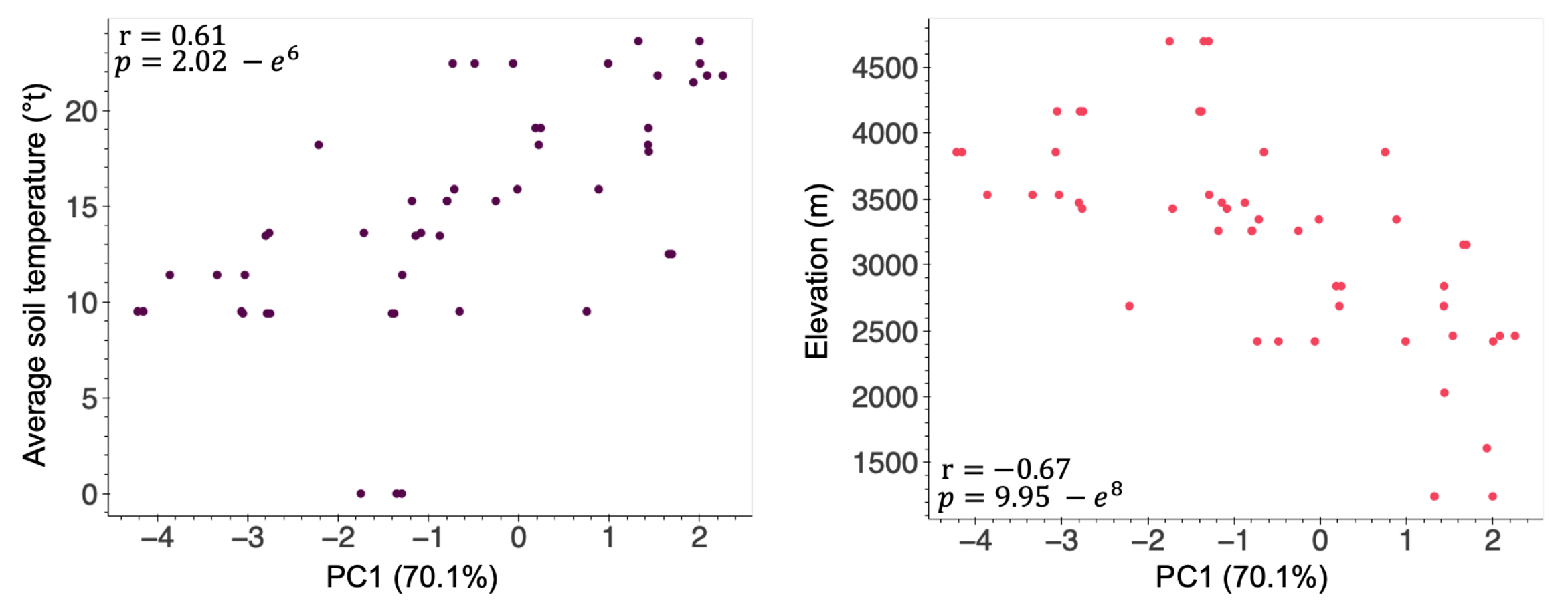
Fig. 18 The first latent component against two measured covariates, from the reference analysis. PC1 tracks average soil temperature (\(r = 0.61\), \(p \approx 2\times 10^{-6}\)) and, more strongly and in the opposite direction, elevation (\(r = -0.67\), \(p \approx 1\times 10^{-7}\)). Each point is one of the 54 samples.

The outcome worth hoping for is a latent axis that stands in for a gradient you measured. Elevation and soil temperature are themselves strongly related along the Atacama transect, so these are two views of one physical gradient rather than two independent findings — PC1 is the transect.

That result says the rank-2 block is absorbing environmental structure rather than batch or library size, which is the check First run set out to make. It does not say the remaining edges are free of environmental confounding: a covariate correlated with a latent axis at \(r = -0.67\) still leaves plenty unexplained. Put elevation into the model explicitly with transform-features --p-add-metadata and compare edge sets, as What to do with the answer describes.

Note

These correlations come from the reference analysis and have not been re-run under QIIME 2 2026.7 — the figure shows what a resolved component-to-covariate assignment looks like, not a verified result for this build. The p-value annotations inside the image are also mis-rendered (2.02 − e6 should read \(2.02\times 10^{-6}\)); the values quoted in the caption above are the correct ones.

Which ASVs load on each axis?

The projection above places samples on the latent axes. The eigenvectors of \(\hat{L}\) place the features: each ASV gets a loading on each axis, and the distribution of those loadings tells you whether an axis is driven by a handful of taxa or by the community as a whole.

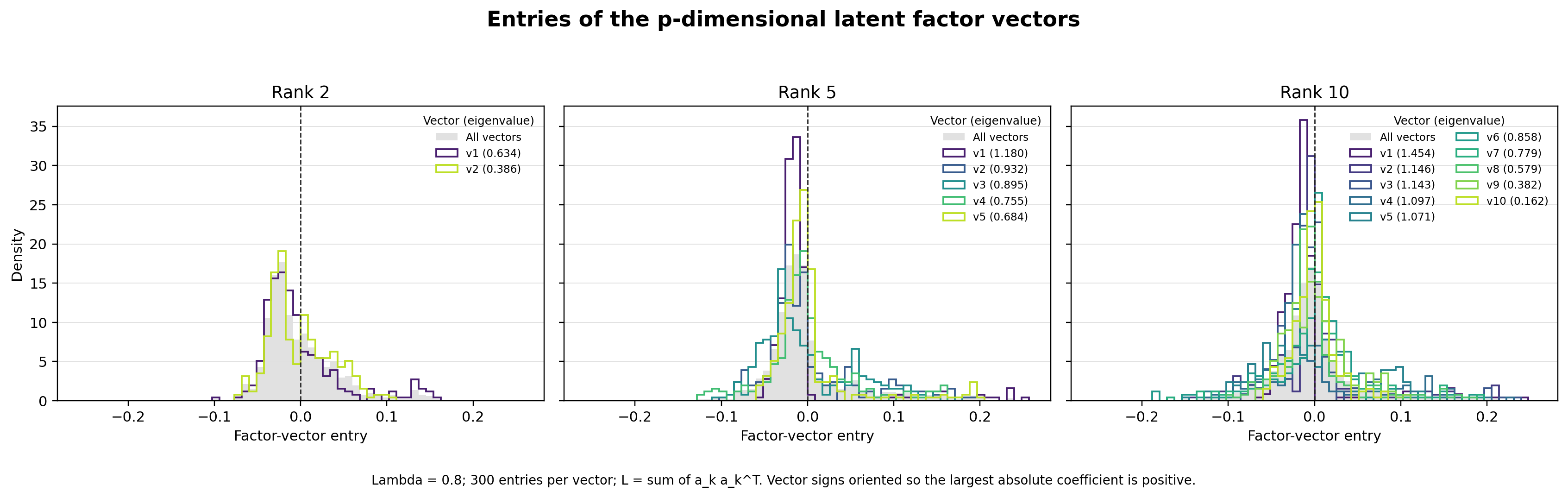
Fig. 19 Per-ASV loadings on the two latent axes at \(\lambda = 0.8\), rank 2. Loadings spread across many ASVs rather than concentrating in a few indicate a community-wide gradient — the signature of an environmental driver rather than a property of one clade.

A broad, roughly symmetric spread is what you expect from a gradient such as pH or moisture acting on the whole community. A spike — most ASVs near zero and a few far out — would instead suggest the axis is tracking something specific, and is worth chasing back to those taxa before calling it environmental.

What to do with the answer

Three outcomes, three next steps.

A component tracks library size — the raw-count total you added to the metadata above, not the seq-depth column the visualizer derives from a clr table. The latent block is absorbing a technical gradient. That is the SLR model doing its job — those directions are no longer contaminating the sparse edges — but it also means that dimension carries no biology, and any statement of the form “there are two latent environmental factors” has to lose one.

A component tracks a measured covariate. You have identified a confounder that you actually measured, which means you no longer have to leave it latent. Append it to the table with transform-features --p-add-metadata and re-fit, as in Adaptive Graphical Lasso, so the variable is in the model explicitly and the remaining edges are conditional on it. Comparing the edge sets before and after is what turns “there is confounding” into “these specific edges were environment-mediated” — Interpretation sets out that comparison.

A component tracks nothing you measured. A candidate unmeasured driver: an unrecorded gradient, a collection batch, an extraction run. It is a hypothesis to take back to the study design, not a finding. This is the case the sparse + low-rank model exists for [M6, M7] — being unable to name the axis does not mean the decomposition failed.

Next

Interpretation puts the sparse block and the latent block back together, and asks whether the latent subspace found here is the same structure the log-contrast models in Log-Contrast Models at Scale are exploiting.