

End-to-End Tutorial#
The workflow below runs both plugins from raw counts to interpreted output, twice: once on a 13-feature table where everything is inspectable by eye, and once on a 300-feature table where it is not. Follow the link at each step when you want the reasoning behind it.
What you need before you start
A working install of both plugins (Installation) and
the tutorial data (Download the Tutorial Data). Everything below assumes the files
sit in data/ and that your QIIME 2 environment is active.
The one idea behind both plugins#
A sequencing run does not measure how much of each taxon is present. It measures proportions, because the total read count per sample is set by the machine and the library preparation, not by biology. Two samples with identical composition but different sequencing depth give different count vectors.
An increase in one taxon’s count therefore forces a decrease in the others, whether or not anything biological changed. Correlations computed on raw counts pick this up as signal, which is why naive co-occurrence networks are full of edges that are artifacts of the constraint rather than of biology.
Both plugins deal with it the same way — they work with log-ratios between features rather than with features themselves. A ratio is unchanged when you rescale a whole sample, so it carries only compositional information.
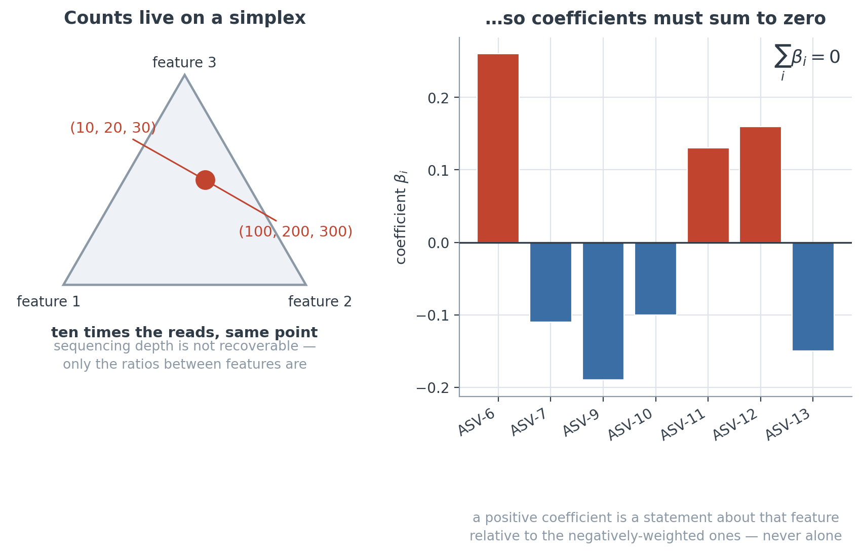
Fig. 3 Sequencing data lives on a simplex — the proportions must sum to one — so features cannot vary independently. Log-ratio transforms map the simplex to ordinary Euclidean space, where standard estimators apply. The zero-sum constraint on log-contrast coefficients is the regression analogue of the same idea.#
From there the two plugins ask different questions of the same table:
Question |
Output |
|
|---|---|---|
q2-gglasso |
Which taxa are related to each other, once every other taxon is accounted for? |
A network of taxon–taxon edges |
q2-classo |
Which combination of taxa predicts an outcome I measured? |
A sparse set of coefficients |
They are not interchangeable. An edge involves no outcome variable; a log-contrast coefficient is a weight inside a zero-sum combination, not a property of one taxon on its own.
Part 1 — Low-dimensional: 13 taxa, 50 samples#
With 13 features and 50 samples there are 78 possible pairs and the sample covariance is full rank and invertible. Penalisation here is a modelling choice, not a necessity — you could fit an unpenalised model, and you can check every number below by hand.
Step 1.1 — Transform the counts#
qiime gglasso transform-features \
    --p-transformation mclr \
    --p-add-metadata False \
    --p-scale-metadata False \
    --i-table data/atacama-counts.qza \
    --i-taxonomy data/classification.qza \
    --m-sample-metadata-file data/selected-atacama-sample-metadata.tsv \
    --o-transformed-table data/atacama-table-mclr.qza
mclr is the modified centred log-ratio: it takes logs of the observed positive
counts and leaves zeros at a common floor below every observed value, rather than
replacing them with an invented number. The alternative, clr, substitutes a
pseudo-count for every zero, and in a typical amplicon table most cells are zero,
so the substitution touches most of the table.
See Data Preparation.
A trap worth knowing now
--i-taxonomy is registered as required but is not read by the transform: the
output is numerically identical whatever valid taxonomy you pass. Pass the correct
file anyway — it costs nothing and you will want it for interpretation.
Step 1.2 — Build the correlation matrix#
qiime gglasso calculate-covariance \
    --p-method scaled \
    --i-table data/atacama-table-mclr.qza \
    --o-covariance-matrix data/atacama-table-corr.qza
scaled divides through by the diagonal, giving a correlation matrix. On a
correlation scale one value of \(\lambda_1\) means roughly the same thing for every
feature pair, which it would not on a covariance scale where high-variance
features dominate.
Step 1.3 — Fit the network#
qiime gglasso solve-problem \
    --p-n-samples 50 \
    --p-lambda1-min 0.001 \
    --p-lambda1-max 1 \
    --p-n-lambda1 50 \
    --p-gamma 0.01 \
    --p-latent False \
    --i-covariance-matrix data/atacama-table-corr.qza \
    --o-solution data/atacama-solution-sgl.qza \
    --verbose
Three parameters carry the modelling decisions:
--p-lambda1-*sweeps the sparsity penalty. Larger \(\lambda_1\) → fewer edges. This is a path, not a single fit: the solver evaluates 50 values and scores each one.--p-gammatunes the model-selection criterion (extended BIC) used to pick among those 50. Higher \(\gamma\) penalises dense graphs more heavily.--p-latent Falsefits a purely sparse model. Part 2 turns this on.
Do not omit the penalty grid
An unset --p-lambda1-* expands to a fifteen-point default path, turning an
intended single fit into a model-selection run at values you did not choose. Always
pass the grid explicitly, and run with --verbose.
Step 1.4 — Read the result#
qiime gglasso summarize \
    --i-solution data/atacama-solution-sgl.qza \
    --p-label-size 25pt \
    --o-visualization data/sgl-summary.qzv
The criterion returns:
\(\gamma\) |
selected \(\lambda_1\) |
edges (of 78 pairs) |
|---|---|---|
0.01 |
0.489 |
1 |
0.10 |
0.489 |
1 |
0.30 |
0.621 |
0 |
0.50 |
0.621 |
0 |
0.70 |
0.621 |
0 |
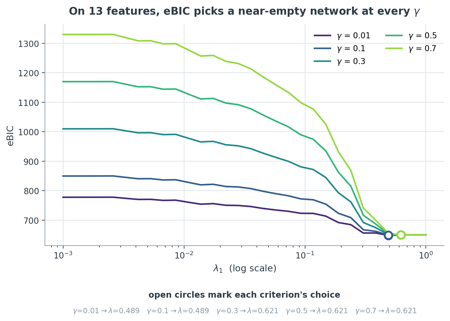
Fig. 4 On 13 features the criterion selects a near-empty network at every \(\gamma\). All five curves decrease monotonically toward the sparse end of the path and the open circles — each criterion’s choice — cluster at \(\lambda_1 \approx 0.5\)–\(0.6\).#
Thirteen abundant taxa across fifty samples do not contain enough conditional-dependence signal for eBIC to prefer a network over no network.
\(\gamma\) barely matters here — every value lands in the same place. That is what changes in Part 2.
Step 1.5 — The same table with q2-classo#
The other question is whether a combination of these taxa predicts soil temperature.
# 1. centred log-ratio, with an adaptive floor for zeros
qiime classo transform-features \
    --p-transformation clr \
    --p-coef 0.5 \
    --i-features data/atacama-counts.qza \
    --o-x data/xclr

# 2. append environmental covariates to the design matrix
qiime classo add-covariates \
    --i-features data/xclr.qza \
    --m-covariates-file data/atacama-selected-covariates-veg.tsv \
    --p-to-add ph average-soil-relative-humidity elevation average-soil-temperature vegetation \
    --p-w-to-add 1. 0.1 0.1 0.1 1 \
    --o-new-features data/xcovariates_lc \
    --o-new-c data/ccovariates_lc \
    --o-new-w data/wcovariates_lc

# 3. hold out 20% for honest error estimation
qiime sample-classifier split-table \
    --i-table data/xcovariates_lc.qza \
    --m-metadata-file data/atacama-selected-covariates-veg.tsv \
    --m-metadata-column average-soil-temperature \
    --p-test-size 0.2 \
    --p-random-state 42 \
    --p-stratify False \
    --o-training-table data/regress-xtraining_lc \
    --o-test-table data/regress-xtest_lc \
    --o-training-targets data/regress-training-targets_lc \
    --o-test-targets data/regress-test-targets_lc

# 4. fit
qiime classo regress \
    --i-features data/regress-xtraining_lc.qza \
    --i-c data/ccovariates_lc.qza \
    --i-weights data/wcovariates_lc.qza \
    --m-y-file data/atacama-selected-covariates-veg.tsv \
    --m-y-column average-soil-temperature \
    --p-concomitant False \
    --p-stabsel \
    --p-cv \
    --p-path \
    --p-lamfixed \
    --p-stabsel-threshold 0.5 \
    --p-cv-seed 1 \
    --p-no-cv-one-se \
    --o-result data/regresstaxa_lc.qza
Two flags in that fit are worth attention.
--i-c is the zero-sum constraint. It is what makes this a log-contrast
model rather than an ordinary regression on transformed features: the coefficients
are forced to sum to zero, so the fit describes ratios between taxa and is
unaffected by rescaling a sample. add-covariates produces the constraint matrix
alongside the design.
--p-stabsel is how you get something interpretable. Selection by itself is
binary and unstable — refit on a slightly different subsample and the chosen set
moves. Stability selection refits many times and reports how often each feature
is chosen, converting a fragile yes/no into a frequency you can rank. With
--p-stabsel-threshold 0.5, features chosen in over half the subsamples are
reported.
A coefficient is not a p-value
Neither plugin provides error control. A non-zero coefficient means “selected at this penalty”, not “significantly non-zero”, and edge counts cannot be compared across studies that used different penalties. Stability frequencies and permutation-based negative controls are the honest substitutes — see Network Interpretation and Analysis.
Full walkthrough: Log-Contrast Regression.
Part 2 — High-dimensional: 300 taxa, 54 samples#
The regime now changes in kind, not just in size. With \(p = 300\) and \(n = 54\), \(p/n = 5.56\) and the sample covariance is singular by construction — its rank cannot exceed \(n - 1 = 53\), so 247 of its 300 eigenvalues are numerically zero. There is no unpenalised model to fall back on. Penalisation is what makes the estimator defined at all.
There are also 44,850 candidate pairs instead of 78, so no result here can be checked by eye. That shifts the burden onto model selection and calibration.
Step 2.1 — Fit a path and let eBIC choose#
qiime gglasso solve-problem \
    --i-covariance-matrix data/atacama-top-300-correlation.qza \
    --p-n-samples 54 \
    --p-no-latent \
    --p-path-scale linear \
    --p-lambda1-min 0.30 --p-lambda1-max 1.00 --p-n-lambda1 15 \
    --p-gamma 0.3 \
    --o-solution data/atacama-top-300-sgl-linear-path.qza
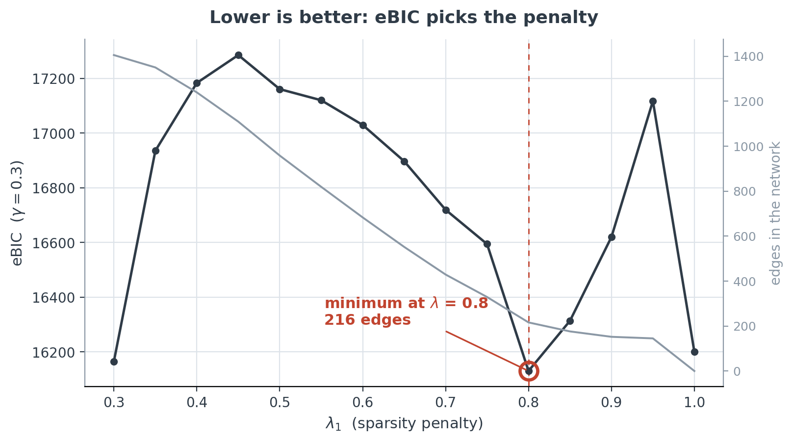
Fig. 5 Model selection on 300 features. The dark curve is eBIC at \(\gamma = 0.3\) (lower is better), minimised at \(\lambda_1 = 0.8\) with 216 edges; the pale curve is edge count on the right axis. Unlike the 13-feature case the criterion has a clear interior minimum, and the curve rises sharply on either side of it.#
The selected model has eBIC 16130.0988 at \(\lambda_1 = 0.8\), giving 216 edges out of 44,850 possible pairs.
gamma is now a decision, not a default
Where \(\gamma\) was irrelevant on 13 features, here it decides the answer: over the conventional range the selected model spans 1405 edges → 216 → the empty graph. Report the \(\gamma\) you used and check the sensitivity around it. The plugin default of 0.01 was reasonable for a small table and is far too permissive at this size. See Choosing the penalties.
Step 2.2 — Separate shared structure from pairwise structure#
A handful of environmental gradients drive many taxa at once. A purely sparse model has no way to represent that, so it charges those broad effects to individual edges. The sparse-plus-low-rank model splits them:
where \(\hat{\Theta}_S\) holds the sparse taxon–taxon edges and \(\hat{L}\) is a low-rank block carrying the shared gradients.
qiime gglasso solve-problem \
    --i-covariance-matrix data/atacama-top-300-correlation.qza \
    --p-n-samples 54 \
    --p-latent \
    --p-lambda1-min 0.8 --p-lambda1-max 0.8 --p-n-lambda1 1 \
    --p-lambda2-min 0.1 --p-lambda2-max 0.1 --p-n-lambda2 1 \
    --p-mu1-min 15 --p-mu1-max 15 --p-n-mu1 1 \
    --o-solution data/atacama-top-300-slr-lambda0.8-rank2.qza
You do not set the rank — you set --p-mu1 and read the achieved rank back from
the solution:
|
achieved rank |
sparse edges |
connected nodes |
|---|---|---|---|
15.0 |
2 |
202 |
162 |
10.0 |
5 |
158 |
124 |
7.5 |
10 |
110 |
92 |
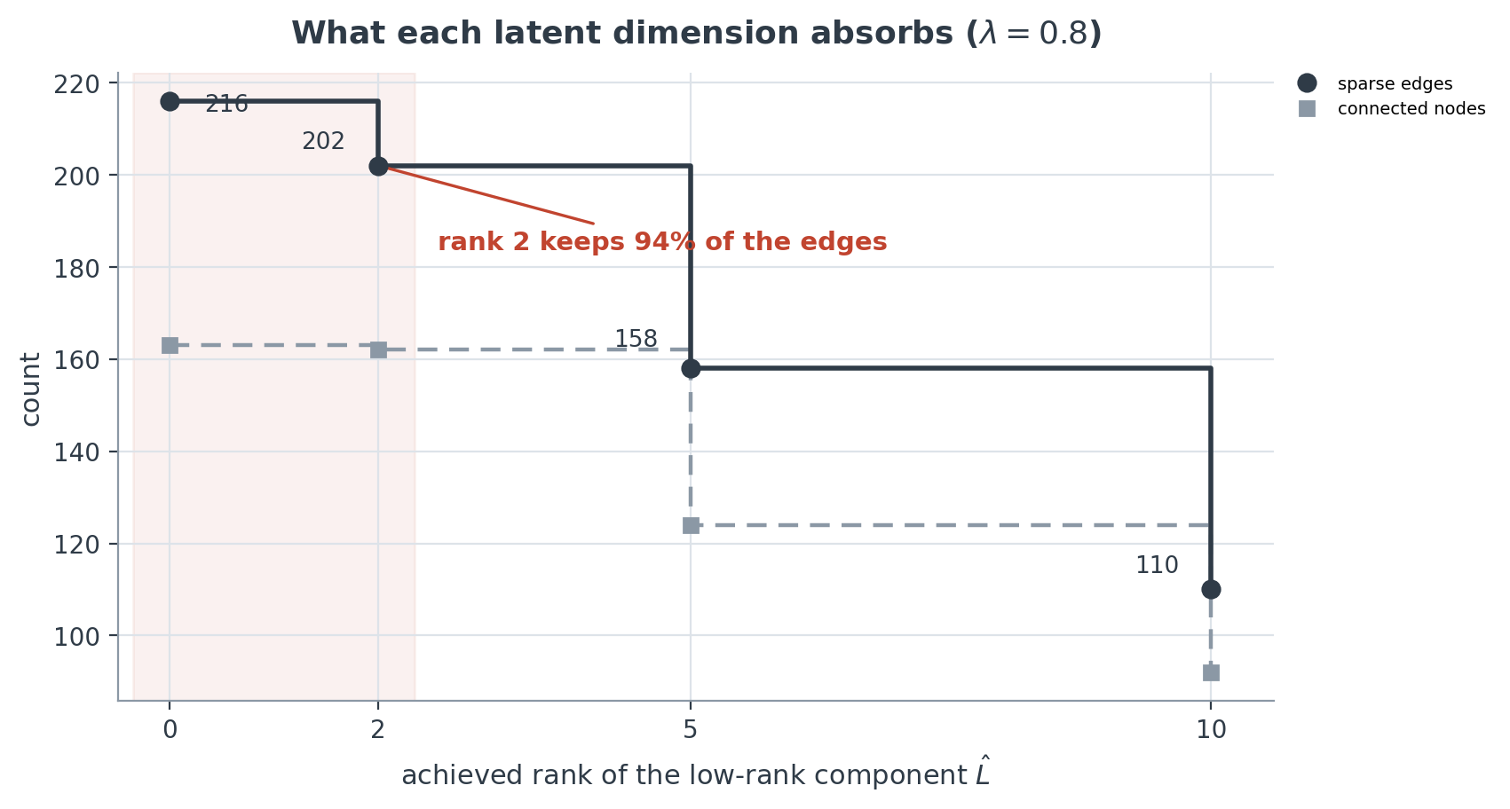
Fig. 6 Every dimension added to \(\hat{L}\) removes edges from the sparse block. Rank 2 keeps 94% of the rank-0 edges; rank 10 keeps half. The shaded region marks the choice made here.#
Comparing the two edge sets directly is the useful diagnostic: 202 edges are
shared, 14 are removed by the latent block, and none are added. That says the 14
removed edges were attributable to shared gradients and the remaining 202 are
not — a stronger statement about those 202 than the sparse-only fit could make.
qiime gglasso summarize reports the edge set for each solution, so you can make
this comparison yourself without drawing a network.
Rank choice: Choosing the Latent Rank. What the latent components correspond to: Latent Components & Covariates.
Step 2.3 — Log-contrast regression at scale#
qiime classo transform-features \
    --i-features data/atacama-top-300-table.qza \
    --o-x data/atacama-top-300-classo-clr.qza

qiime classo regress \
    --i-features data/atacama-top-300-classo-clr.qza \
    --m-y-file data/atacama-classo-outcomes-mean-imputed.tsv \
    --m-y-column average-soil-temperature \
    --p-cv --p-cv-subsets 5 --p-cv-seed 1 --p-cv-one-se \
    --p-cv-nlam 60 --p-cv-lamin 0.001 --p-cv-logscale \
    --o-result data/average-soil-temperature-cv5.qza
At this scale cross-validation replaces a fixed penalty: --p-cv-subsets 5 splits
the data five ways and --p-cv-one-se applies the one-standard-error rule, which
prefers the sparsest model within one standard error of the best. That is a
deliberate bias toward parsimony and standard practice; state it in any methods
description that relies on the fit.
Across 15 environmental outcomes the fits select between 1 and 33 of the 300
features. Three outcomes (depth, ec, toc) select a single feature, which is
the model saying it found nothing usable rather than finding one decisive taxon.
Check your outcome column before you trust the fit
In this metadata ph = 0 is a missing-value sentinel for 8 samples — roughly 2.8
standard deviations below the mean — and it enters the regression as a real
measurement. Sentinel-coded missingness is common in field metadata and silently
distorts any fit that uses it. Look at your outcome’s distribution first.
Full treatment: High-Dimensional Example: q2-classo on 300 Atacama ASVs.
The two regimes compared#
13 taxa, 50 samples |
300 taxa, 54 samples |
|
|---|---|---|
\(p/n\) |
0.26 |
5.56 |
Covariance |
full rank, invertible |
singular; rank \(\le 53\) |
Penalisation is |
a modelling choice |
what defines the estimator |
Candidate pairs |
78 |
44,850 |
eBIC selects |
1 edge, or none |
216 edges |
Effect of \(\gamma\) |
negligible |
1405 → 216 → 0 edges |
Verification |
inspect the matrix |
model selection and calibration |
The last row is the transferable one. On a small table you can look at the answer and judge it. On a high-dimensional table you cannot, so the penalty, the selection criterion and its sensitivity are the result. Report them alongside the network.
Reproducing the results#
Every figure and number here regenerates from committed inputs, with no cluster and no QIIME 2 installation:
git clone https://github.com/Vlasovets/q2-hdstats-docs
cd q2-hdstats-docs
pip install -r analysis/requirements-figures.txt
python analysis/scripts/make_docs_figures.py
The inputs are 103 KB of TSV under analysis/results/. To rebuild this book
locally:
pip install -r requirements.txt
jupyter-book build docs --warningiserror
To re-run the qiime commands themselves you need the plugin environments, which
solve everything in one conda transaction:
file |
what it pins |
|---|---|
|
the fully solved analysis environment |
|
q2-gglasso + QIIME 2 2026.7 |
|
q2-classo + QIIME 2 2026.7 |
|
figure generation only, no QIIME 2 |
|
re-capturing the plugin visualizations from the committed |
|
the documentation toolchain |
Provenance for every input file — sizes and SHA-256 digests — is in
docs/_data/manifest.tsv.
Data availability
Eleven of the sixteen manifest rows currently read ZENODO_DOI_PENDING: the files
are committed under analysis/publish/ and verified against the manifest, but the
archival deposit is not yet minted. The five gut-to-soil rows carry live upstream
URLs. Until the deposit exists, obtain the tutorial files as described in
Download the Tutorial Data.
Where to go next#
Every parameter of either plugin — q2-gglasso Parameter Reference and q2-classo Parameter Reference
Which chapter owns which command — Command Coverage Matrix
Errors and their causes — Troubleshooting & Known Failure Modes
The mathematics — Appendix: Mathematical Background