Tree-Aggregated Regression (trac)

Log-Contrast Regression treated the 13 ASVs as 13 unrelated predictors. They are not unrelated — they sit in a taxonomy, and two ASVs in the same genus are far more likely to respond to soil temperature the same way than two from different phyla.

trac [C4] uses that structure. Instead of selecting individual ASVs it can select an internal node — a genus, an order, a phylum — and use the aggregated abundance of everything beneath it. That changes what the result says: “Nitriliruptorales predicts temperature” is more useful and more testable than a list of four ASV hashes that happen to belong to it.

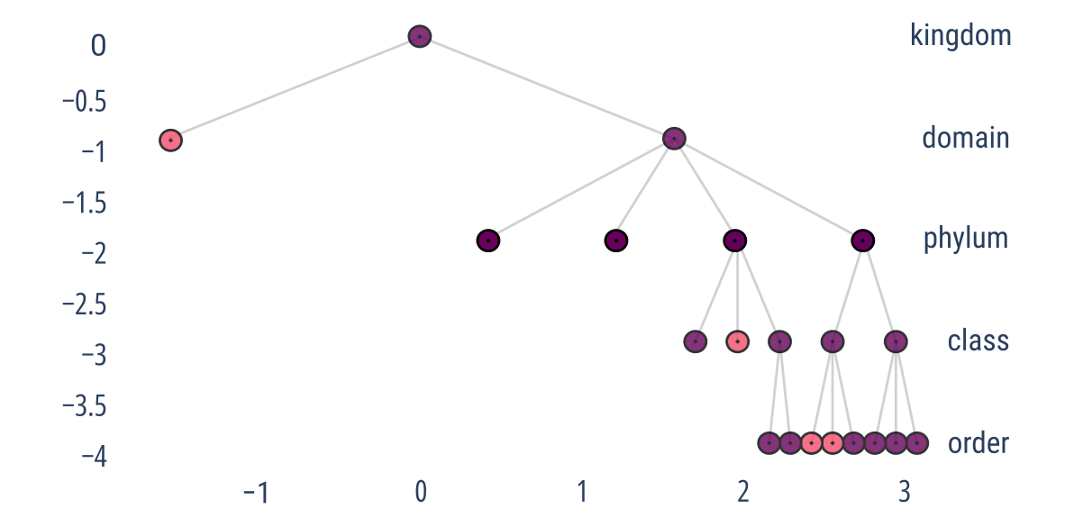
Fig. 12 The taxonomy trac aggregates over. Each level is a rank, each node a taxon, and trac may place a coefficient on any node, not only on the leaves. Selecting a node high in the tree is a claim about a whole clade. Selecting a leaf is a claim about one ASV.

Note

Ignore the axis numbers: they are layout coordinates from the plotting routine, not data. The top row is labelled “kingdom”, but the SILVA 138 taxonomy used here has no kingdom rank — its strings run d__ (domain), p__, c__, o__, f__, g__, s__. That row is the tree’s artificial root, and the row below it, “domain”, is d__Bacteria.

Step 1: Transform Features

Apply CLR transformation to the count data:

qiime classo transform-features \
    --p-transformation clr \
    --p-coef 0.5 \
    --i-features data/atacama-counts.qza \
    --o-x data/xclr

Step 2: Add Taxonomic Information

Attach the taxonomy to the design and derive an adaptive weight for every node:

qiime classo add-taxa \
    --i-features data/xclr.qza  \
    --i-taxa data/classification.qza \
    --o-x data/xtaxa \
    --o-aweights data/wtaxa

The action uses the taxonomic hierarchy to structure the relationships between features and derives each adaptive weight from the taxonomic distances, which encourages the fit to select taxa that share taxonomic relatives.

Step 3: Add Covariates

Include environmental metadata with custom weights, alongside the taxonomic features:

qiime classo add-covariates \
    --i-features data/xtaxa.qza \
    --i-weights data/wtaxa.qza \
    --m-covariates-file data/atacama-selected-covariates-veg.tsv \
    --p-to-add ph average-soil-relative-humidity elevation average-soil-temperature vegetation \
    --p-w-to-add 1. 0.1 0.1 0.1 1 \
    --o-new-features data/xcovariates_trac \
    --o-new-c data/ccovariates_trac \
    --o-new-w data/wcovariates_trac

Step 4: Split Data

Create training and test sets for regression analysis:

qiime sample-classifier split-table \
    --i-table data/xcovariates_trac.qza \
    --m-metadata-file data/atacama-selected-covariates-veg.tsv \
    --m-metadata-column average-soil-temperature \
    --p-test-size 0.2 \
    --p-random-state 42 \
    --p-stratify False \
    --o-training-table data/regress-xtraining_trac.qza \
    --o-test-table data/regress-xtest_trac.qza \
    --o-training-targets data/regress-training-targets_trac.qza \
    --o-test-targets data/regress-test-targets_trac.qza

Step 5: Train the Regression Model

Fit the model on the aggregated design, with stability selection alongside it:

qiime classo regress \
    --i-features data/regress-xtraining_trac.qza \
    --i-c data/ccovariates_trac.qza \
    --i-weights data/wcovariates_trac.qza \
    --m-y-file data/atacama-selected-covariates-veg.tsv \
    --m-y-column average-soil-temperature \
    --p-concomitant False \
    --p-stabsel \
    --p-cv \
    --p-path \
    --p-lamfixed \
    --p-stabsel-threshold 0.5 \
    --p-cv-seed 1 \
    --p-no-cv-one-se \
    --o-result data/regresstaxa_trac.qza

Key parameters:

• --p-stabsel: Run stability selection alongside the path fit

• --p-stabsel-threshold 0.5: Keep features selected in more than 50% of subsamples

• --p-cv: Choose the penalty by cross-validation

• --p-concomitant False: Hold the noise scale fixed rather than estimating it

Step 6: Make Predictions

Apply the trained model to test data:

qiime classo predict \
    --i-features data/regress-xtest_trac.qza \
    --i-problem data/regresstaxa_trac.qza \
    --o-predictions data/regress-predictions_trac.qza

Step 7: Visualize Results

Render the fit, the taxonomy and the predictions as a single report:

qiime classo summarize \
    --i-problem data/regresstaxa_trac.qza \
    --i-taxa data/classification.qza \
    --i-predictions data/regress-predictions_trac.qza \
    --o-visualization data/regresstaxa_R1_trac.qzv

The .qzv file contains:

• the selected taxa with their taxonomic context

• model performance metrics (R², RMSE, and others)

• taxonomic group importances

• cross-validation curves

• prediction accuracy on the test data

View the results at QIIME 2 View.

Log-contrast and trac side by side

Log-contrast treats each taxon as an independent predictor, fits faster, and suits exploratory work.

trac uses the taxonomic relationships, reports coefficients on named clades, selects features better when the structure is hierarchical, and takes somewhat longer to fit.