

Interpreting Log-Contrast Models#
What the coefficients describe#
A log-contrast model works on log-ratios, which is what lets it fit data constrained to sum to a constant. Read the taxon coefficients it reports as statements about ratios between taxa rather than about abundances.
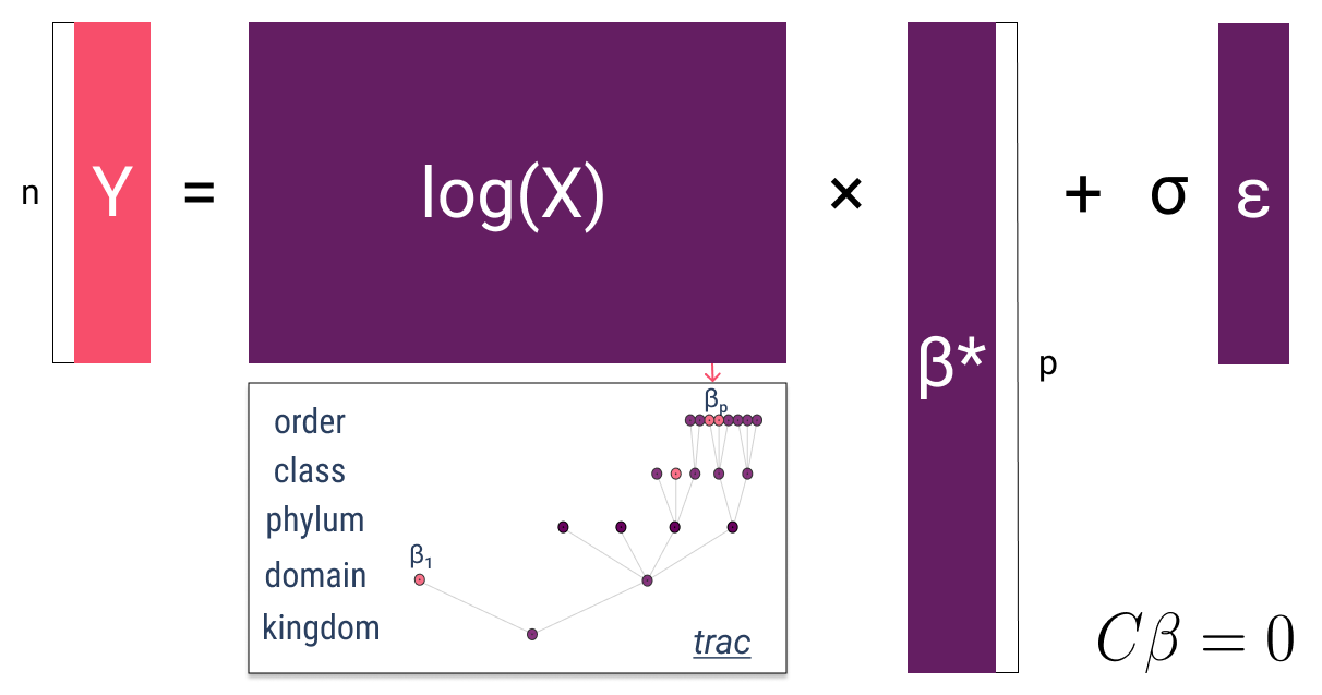
Fig. 15 The whole log-contrast model in one line. The outcome \(Y\) (\(n\) values) is
regressed not on the counts but on \(\log(X)\), against a coefficient vector
\(\beta^*\) of length \(p\), plus noise scaled by \(\sigma\) — the scale that
--p-concomitant estimates jointly rather than fixing.#
The two annotations are what make it compositional. \(C\beta = 0\) at the
bottom right is the zero-sum constraint: the coefficients must sum to zero,
so the fit depends only on ratios between taxa and is unchanged if every
sample is rescaled. That is what removes the arbitrary sequencing depth. The
inset shows the trac variant, where the constraint matrix \(C\) encodes the
taxonomic tree — coefficients attach to internal nodes from kingdom up to
order, so a single \(\beta\) can act on a whole clade instead of one ASV.
Regression#
A regression predicts a continuous outcome from the composition, and each coefficient carries the effect of one log-ratio on that outcome:
A unit change in the log-contrast moves the predicted outcome by the coefficient
A positive coefficient suggests that a higher abundance of the numerator taxa relative to the denominator taxa is associated with higher predicted values
The denominator taxa are the reference for every comparison
Classification#
A classification predicts a categorical outcome from the same predictors, with the decision boundary drawn in log-ratio space:
The features that carry weight are the log-contrasts that separate the classes
Class probabilities are computed in the transformed space
Read the result as a statement about relative abundance, not absolute abundance
Model-selection procedures help assess how reliable the model is across different compositional profiles