

Regularization Paths & Model Selection#
Every chapter so far has handed solve-problem a range of \(\lambda_1\) values and
accepted whatever came back. The plugin makes two decisions with that range:
Which values are tried — the regularization path, built from
lambda1_min/lambda1_max/n_lambda1and the spacing rulepath_scale, or supplied verbatim throughlambda1_path.Which value is kept — the extended BIC (eBIC), whose behaviour is controlled by a single parameter,
gamma.
Get either one wrong and the failure is quiet: you still get a solution artifact, but not the one you thought you asked for. The same machinery runs on 300 features in Selecting lambda, where the choice changes the biology.
How the grid is built#
For each penalty, solve-problem builds a grid from three numbers and a spacing
rule. With --p-path-scale log (the default) the grid is log-spaced between the
bounds; with --p-path-scale linear it is evenly spaced. The same
path_scale applies to \(\lambda_1\), \(\lambda_2\) and \(\mu_1\) — there is one
spacing rule per invocation, not one per penalty.
Three behaviours of the grid builder do not follow from the flag names:
Omitting one bound does not omit the grid. If you give lambda1_min but not
lambda1_max, the missing upper bound silently becomes 1; a missing lower
bound becomes 1e-3. You get a full grid built against a default endpoint you
never chose.
Omitting both bounds gives you a default path, not a single fit. When both ends of a penalty range are unset, the plugin substitutes a built-in path and emits a warning:
Penalty |
Default path when both bounds are unset |
Values |
|---|---|---|
\(\lambda_1\) |
|
15, from |
\(\lambda_2\) |
|
5, from |
\(\mu_1\) (only when |
|
10, from |
Each substitution prints a warning of the form “Default values for lambda1 have
been used.” — run with --verbose or you will not see it.
An explicit path wins over everything. --p-lambda1-path and
--p-mu1-path take a list of values that is used exactly as given. They
override *_min, *_max, n_* and path_scale. There is no lambda2_path.
Express a hand-built \(\lambda_2\) grid through lambda2_min / lambda2_max /
n_lambda2.
Note
Neither plugin declares Choices() on its string parameters, so
--p-path-scale logg is accepted by the command line and fails inside the
function with ValueError: Unknown scale 'logg', use 'log' or 'linear'.
See Troubleshooting.
Single fit versus model selection#
solve-problem runs a model-selection search whenever any relevant grid holds
more than one value. The rule reads the final grids, after the defaults above
have been substituted, and which grids it consults depends on latent:
Without
--p-latent: a single fit requires that the \(\lambda_1\) grid and the \(\lambda_2\) grid each hold exactly one value. The \(\mu_1\) grid is not consulted.With
--p-latent: a single fit requires that \(\lambda_1\), \(\lambda_2\) and \(\mu_1\) each hold exactly one value. All three.
Read that together with the default-path rule above: leaving \(\lambda_2\) unset does not make it a singleton. The plugin replaces an unset \(\lambda_2\) range with the five-value default path, so the grid holds more than one value and model selection runs whatever you did to \(\lambda_1\). On a single-instance problem \(\lambda_2\) has no effect on the answer, but it still decides which branch runs. Pin it explicitly to get one fit.
The latent case catches people. Pin \(\lambda_1\) to one value, leave \(\mu_1\) unset, and you do not get one model at that \(\lambda_1\): the \(\mu_1\) default path supplies ten values, model selection runs, and eBIC is free to move away from the \(\lambda_1\) you thought you had fixed. Pin all three to fit exactly one latent model:
# exactly one model: one lambda1, one lambda2, one mu1
qiime gglasso solve-problem \
    --i-covariance-matrix data/atacama-table-corr.qza \
    --p-n-samples 50 \
    --p-latent True \
    --p-lambda1-min 0.1 --p-lambda1-max 0.1 --p-n-lambda1 1 \
    --p-lambda2-min 0.1 --p-lambda2-max 0.1 --p-n-lambda2 1 \
    --p-mu1-min 0.5 --p-mu1-max 0.5 --p-n-mu1 1 \
    --o-solution data/atacama-solution-single-fit.qza \
    --verbose
Note
--p-n-samples 50 matches the value used by the other Tier 1 chapters. It must
equal the number of samples behind the covariance matrix, and for the 13-ASV
subset that count is settled: the table is 13 features × 50 samples, read
directly off the artifact (see
Downloading the Data). On your own
table, read the count off your qiime feature-table summarize output rather than
copying a published number.
To find out which branch ran, look for a modelselect_stats group in the
solution: a single fit has none, and
summarize omits the statistics accordingly.
The same problem, three ways#
The three runs below differ only in how the \(\lambda_1\) path is constructed.
Everything else — the covariance matrix, the sample count, gamma, the absence
of latent variables — is held fixed, so any difference in the selected model is
attributable to the path alone.
A. Log-spaced (the default). Fifteen values between 0.001 and 1, each
about 1.64× the previous one:
qiime gglasso solve-problem \
    --i-covariance-matrix data/atacama-table-corr.qza \
    --p-n-samples 50 \
    --p-latent False \
    --p-lambda1-min 0.001 --p-lambda1-max 1 --p-n-lambda1 15 \
    --p-path-scale log \
    --p-gamma 0.01 \
    --o-solution data/atacama-solution-path-log.qza \
    --verbose
B. Linearly spaced. Same endpoints, same number of points, uniform steps of
about 0.071:
qiime gglasso solve-problem \
    --i-covariance-matrix data/atacama-table-corr.qza \
    --p-n-samples 50 \
    --p-latent False \
    --p-lambda1-min 0.001 --p-lambda1-max 1 --p-n-lambda1 15 \
    --p-path-scale linear \
    --p-gamma 0.01 \
    --o-solution data/atacama-solution-path-linear.qza \
    --verbose
C. An explicit path. Ten values chosen by hand; path_scale is ignored:
qiime gglasso solve-problem \
    --i-covariance-matrix data/atacama-table-corr.qza \
    --p-n-samples 50 \
    --p-latent False \
    --p-lambda1-path 1.0 0.5 0.25 0.1 0.05 0.025 0.01 0.005 0.0025 0.001 \
    --p-gamma 0.01 \
    --o-solution data/atacama-solution-path-explicit.qza \
    --verbose
Nine of the fifteen log-spaced values in run A lie below the second linear
value in run B (≈0.072), so run A spends most of its grid on weak penalties
and dense networks and run B most of its grid on the sparse end. If the eBIC
optimum sits near \(\lambda_1 = 0.01\), run B cannot find it — its nearest grid
point is an order of magnitude away. Conversely, if the optimum sits near
\(\lambda_1 = 0.6\), run A has only two candidates above it.
Give an explicit path when you already know roughly where the optimum lies and want a reproducible, human-readable grid in the provenance record rather than a triple of bounds that a reader has to re-derive.
Note
These three runs have not yet been recomputed against QIIME 2 2026.7, so the selected \(\lambda_1\), the eBIC value and the resulting edge counts are not quoted here.
Comparing the three selections#
Visualize each solution and compare them on three axes:
qiime gglasso summarize \
    --i-solution data/atacama-solution-path-log.qza \
    --p-label-size 25pt \
    --o-visualization data/path-log-summary.qzv

qiime gglasso summarize \
    --i-solution data/atacama-solution-path-linear.qza \
    --p-label-size 25pt \
    --o-visualization data/path-linear-summary.qzv

qiime gglasso summarize \
    --i-solution data/atacama-solution-path-explicit.qza \
    --p-label-size 25pt \
    --o-visualization data/path-explicit-summary.qzv
The selected \(\lambda_1\). If the three runs land on values that are close in absolute terms, the optimum is well identified and the path only affects precision. If they land in different regimes, the eBIC surface is flat and you are choosing a model by grid design, not by evidence.
The sparsity level. Two paths can select different \(\lambda_1\) values and still produce nearly the same network. Edge count is the quantity you care about, and \(\lambda_1\) is only the dial that produces it.
Where the optimum sits on the path. An optimum at the first or the last grid point means the search range was too narrow.
Important
If the selected \(\lambda_1\) is the smallest or largest value on the path,
solve-problem emits two warnings — a directional one naming the fix, followed
by a general one:
lambda is on the edge of the interval, try SMALLER lambda1
lambda is on the edge of the interval, the solution might have not reached global minimum!
(try BIGGER lambda1 when the selection sits at the top of the range.) A
selection at either end means the optimum lies outside the range you searched.
Widen the bounds in the direction named and re-run.
The boundary test covers \(\lambda_1\) and, for multiple-instance problems,
\(\lambda_2\). There is no equivalent check on \(\mu_1\), so a latent solution can
select the smallest or largest \(\mu_1\) on your path with no warning at all.
Read the selected \(\mu_1\) out of summarize yourself and
confirm it is interior.
gamma and the extended BIC#
Model selection scores each fitted model with the extended BIC of Foygel and Drton [M2]. Ordinary BIC penalizes the number of edges; the extended version adds a second penalty term scaled by \(\gamma \in [0, 1]\) that accounts for the size of the model space. Larger \(\gamma\) means a heavier penalty on extra edges, hence a sparser selection.
Three values appear across these chapters:
\(\gamma\) |
Where it is used |
Character |
|---|---|---|
|
the plugin default, and every Tier 1 chapter |
almost plain BIC; the most permissive of the three |
|
the 300-ASV analysis in Selecting lambda |
a deliberate middle ground for a high-dimensional problem |
|
the conventional choice in the eBIC literature |
conservative; the usual default elsewhere |
Re-running the log path under all three makes the sensitivity visible:
qiime gglasso solve-problem \
    --i-covariance-matrix data/atacama-table-corr.qza \
    --p-n-samples 50 --p-latent False \
    --p-lambda1-min 0.001 --p-lambda1-max 1 --p-n-lambda1 15 \
    --p-gamma 0.01 \
    --o-solution data/atacama-solution-gamma-001.qza

qiime gglasso solve-problem \
    --i-covariance-matrix data/atacama-table-corr.qza \
    --p-n-samples 50 --p-latent False \
    --p-lambda1-min 0.001 --p-lambda1-max 1 --p-n-lambda1 15 \
    --p-gamma 0.3 \
    --o-solution data/atacama-solution-gamma-03.qza

qiime gglasso solve-problem \
    --i-covariance-matrix data/atacama-table-corr.qza \
    --p-n-samples 50 --p-latent False \
    --p-lambda1-min 0.001 --p-lambda1-max 1 --p-n-lambda1 15 \
    --p-gamma 0.5 \
    --o-solution data/atacama-solution-gamma-05.qza
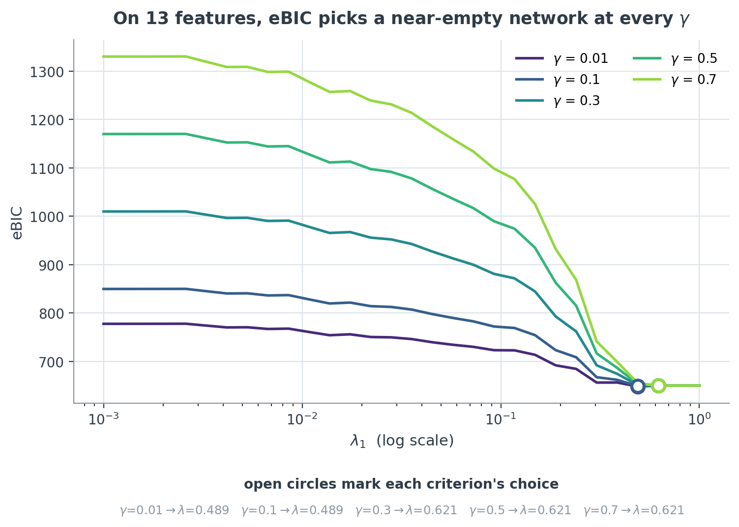
Fig. 8 eBIC against \(\lambda_1\) on the 13-ASV table, scored at five values of \(\gamma\). Open circles mark each criterion’s choice. The curves separate vertically — a larger \(\gamma\) charges more for the same model — but they are minimised at almost the same place, so the five criteria between them pick only two distinct \(\lambda_1\) values.#
Generated by analysis/slurm/30_tier1_figures.sh from a single 30-point path,
not from the three commands above: GGLasso scores every candidate model under a
fixed internal set of \(\gamma\), so one solve-problem run already carries all
five curves in modelselect_stats/BIC. The three-command form gives one
selected solution per \(\gamma\); run at 15 grid points it lands on neighbouring
\(\lambda_1\) values rather than these exact ones.
On this dataset \(\gamma\) barely matters. The five criteria collapse onto two adjacent grid points, and both of those networks are all but empty:
\(\gamma\) |
selected \(\lambda_1\) |
edges (of 78 possible) |
|---|---|---|
0.01, 0.1 |
0.4894 |
1 |
0.3, 0.5, 0.7 |
0.6210 |
0 |
With 13 features and 50 samples the problem is not high-dimensional, eBIC’s model-space penalty has little to bite on, and the criterion is decisive well before \(\gamma\) gets a say. Turning \(\gamma\) up from 0.01 to 0.7 costs you the single surviving edge. The Tier 1 chapters therefore mostly show fits at a fixed \(\lambda_1\): on a table this small, letting eBIC choose returns an empty graph.
Contrast the 300-ASV Atacama analysis, where \(p = 300\) and \(n = 54\). There the same parameter flips the answer between 1405 edges, 216 edges and the empty graph across the window \(\gamma \in [0.29, 0.32]\) — three qualitatively different scientific conclusions, a hundredth apart.
gamma does nothing at all in a single fit: only the model-selection routine
consumes it, so pinning every grid to one value makes the flag inert. Where
selection does run, gamma is a modelling choice on the level of a significance
threshold. Report it with any network you derive from it — a network published
without its \(\gamma\) is not reproducible, and the two cases above show that you
cannot predict from the value alone whether it mattered.
Tip
Do not tune gamma until you are satisfied with the path. A gamma sweep on a
grid whose optimum sits at the boundary tells you about the grid, not about the
data.
Latent paths: the \(\mu_1\) dimension#
With --p-latent there is a second path to design. --p-mu1-min,
--p-mu1-max and --p-n-mu1 build it from bounds under the shared
path_scale; --p-mu1-path supplies it verbatim and overrides all three. The
search is over the product of the \(\lambda_1\) and \(\mu_1\) grids, so a 15 × 10
specification is 150 fits — cheap on 13 features, much less so on 300.
# scout a coarse mu1 path at a fixed lambda1
qiime gglasso solve-problem \
    --i-covariance-matrix data/atacama-table-corr.qza \
    --p-n-samples 50 \
    --p-latent True \
    --p-lambda1-min 0.1 --p-lambda1-max 0.1 --p-n-lambda1 1 \
    --p-lambda2-min 0.1 --p-lambda2-max 0.1 --p-n-lambda2 1 \
    --p-mu1-path 10.0 5.0 2.0 1.0 0.5 0.2 \
    --p-gamma 0.01 \
    --o-solution data/atacama-solution-mu1-scout.qza \
    --verbose
\(\mu_1\) controls the rank of the low-rank component: a larger \(\mu_1\) yields a
smaller rank. It is the only handle available — --p-rank is registered but
never works: without --p-latent it raises ValueError (“the rank parameter
is only meaningful for the sparse + low-rank model”), and with --p-latent it
raises NotImplementedError on every released GGLasso up to and including
0.3.0, because no release can fix the rank directly. Scout a \(\mu_1\) path and
read the achieved rank out of each solution; see
Sparse + Low-Rank and, at scale,
Choosing the Latent Rank.
A practical recipe#
Start wide and log-spaced:
--p-lambda1-min 0.001 --p-lambda1-max 1 --p-n-lambda1 15. Log spacing is the right default because the interesting behaviour of an L1 penalty is multiplicative.Run with
--verboseand read the warnings. A “default values have been used” warning means you did not specify the grid you thought you did.Check that the selection is interior, not at a boundary. Widen and re-run if it is not.
Refine with a narrower path — or an explicit
--p-lambda1-path— around the optimum.Only then vary
gamma, and report the value you settled on.For latent models, pin \(\lambda_1\) and \(\lambda_2\) while scouting \(\mu_1\); leaving any of the three unpinned re-enables the full search.
The full parameter list, with types and defaults, is in the q2-gglasso Parameter Reference.