Adding latent variables

Single Graphical Lasso assumes that everything driving the correlations between these 13 ASVs is one of the 13 ASVs. That is rarely true of soil. Moisture, pH and depth act on many taxa at once, and a driver left out of the model has nowhere to put its footprint except the edges — weak associations between taxa that share a habitat rather than an interaction.

The sparse + low-rank model estimates that footprint separately. It splits the precision matrix into two pieces, fitted together:

\[\hat{\Theta} = \underbrace{\hat{\Theta}_S}_{\text{sparse: the network}} - \underbrace{\hat{L}}_{\text{low rank: a few global directions}}\]

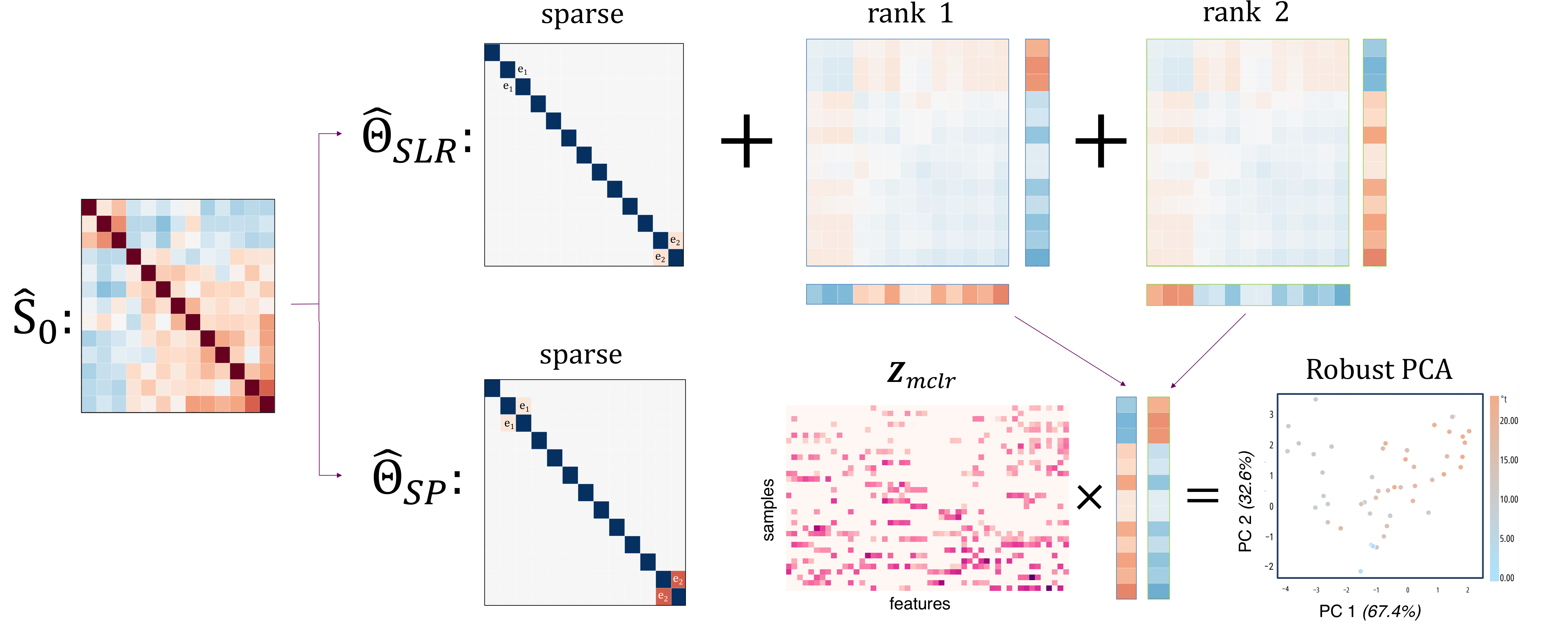
Fig. 7 The decomposition. From the empirical covariance \(\hat{S}_0\) (left), the SLR model estimates a sparse block plus a small number of rank-one directions, while the sparse-only model \(\hat{\Theta}_{SP}\) must absorb everything into edges. The eigenvectors of the low-rank block project the samples — that projection is the robust PCA on the right, and is what Latent-Component PCA plots.

The sparsity penalty \(\lambda_1\) still controls how many edges survive. A second penalty, \(\mu_1\), controls how much structure the low-rank block may absorb: a larger \(\mu_1\) permits fewer latent directions.

Fitting the model

qiime gglasso solve-problem \
    --p-n-samples 50 \
    --p-lambda1-min 0.001 --p-lambda1-max 1 --p-n-lambda1 50 \
    --p-mu1-min 0.50118723 --p-mu1-max 0.79432823 --p-n-mu1 50 \
    --p-gamma 0.01 \
    --p-latent True \
    --i-covariance-matrix data/atacama-table-corr.qza \
    --o-solution data/atacama-solution-slr.qza \
    --verbose

--p-latent True turns this into an SLR problem. Without it the mu1 grid is ignored. Both grids are searched jointly and scored by eBIC, so this one command is a model-selection run over \(50 \times 50\) combinations, not a single fit. The remaining arguments are the ones described in Single Graphical Lasso.

The selected model

The solution artifact records:

quantity	value
features	13
selected \(\lambda_1\)	0.2442
selected \(\mu_1\)	0.7722
achieved rank of \(\hat{L}\)	2
edges in \(\hat{\Theta}_S\)	4 of 78 possible pairs
eigenvalues of \(\hat{L}\)	0.761, 0.151, 0, 0, …

Three properties of this solution:

A lopsided latent block. The rank is 2, and the two non-zero eigenvalues are 0.761 and 0.151, so the first latent direction carries 83% of the low-rank energy: one dominant global gradient with a weaker second one, which is what you would expect from a transect study, and what Latent-Component PCA will let you plot.

A very sparse network. Four edges among 13 ASVs. With \(n = 50\) samples and 78 possible pairs the problem is small, and eBIC at \(\gamma = 0.01\) is not being generous. Do not read the absence of an edge as evidence of independence at this sample size.

The rank is an output rather than a setting. You chose a \(\mu_1\) range. The model chose 2. There is no --p-rank to set it directly — see Choosing the Latent Rank for how to steer \(\mu_1\) toward a target rank when you need one.

Important

“SLR gives fewer edges than SGL” is false on this dataset.

Running the sparse-only model on the identical covariance matrix gives:

model	selected \(\lambda_1\)	edges
SGL (--p-no-latent)	0.4292	2
SLR (--p-latent)	0.2442	4

SLR found more edges, because each model selects its own penalty and SGL selected a much heavier one. The intuition that a latent block removes edges holds at a fixed \(\lambda_1\), where the low-rank component absorbs correlation that would otherwise be spent on edges. The 300-ASV example is the fixed-penalty case: at \(\lambda = 0.8\), adding two latent dimensions takes the network from 216 edges to 202 and adds none (Interpretation).

When the penalties differ, edge counts are not comparable. Compare at fixed \(\lambda_1\), or compare the selected models as models — not by counting edges.

Visualising the decomposition

qiime gglasso summarize \
    --i-solution data/atacama-solution-slr.qza \
    --p-label-size 25pt \
    --o-visualization data/slr-summary.qzv

The .qzv carries a Low-rank tab that the SGL summary does not, showing \(\hat{L}\) as a heatmap alongside the sparse block. Open it with qiime tools view or at QIIME 2 View, and check the Statistics tab against the table above — the selected \(\lambda_1\), \(\mu_1\) and rank are recorded there.

Outputs

data/atacama-solution-slr.qza holds a 4-edge network and a rank-2 latent block, the two estimated jointly rather than in sequence. Latent-Component PCA projects the samples onto the eigenvectors of \(\hat{L}\). Interpretation reads the sparse block as a network.