Log-Contrast Regression

Can the community predict the soil temperature it lives in, and which taxa carry that signal?

That is a regression with a constraint. The predictors are compositional: sequencing depth is arbitrary, so only ratios between features mean anything. Log-contrast regression transforms to log-ratios and requires the coefficients to sum to zero, so the fit depends on the balance between taxa rather than on any absolute abundance the sequencing run happened to produce [C2, C3].

This fit uses no taxonomy. Tree-Aggregated Regression puts it back, and the two are worth comparing.

Step 1: Transform Features

Apply CLR transformation to the count data:

qiime classo transform-features \
    --p-transformation clr \
    --p-coef 0.5 \
    --i-features data/atacama-counts.qza \
    --o-x data/xclr

Step 2: Add Covariates

Include environmental metadata with custom weights for each covariate:

qiime classo add-covariates \
    --i-features data/xclr.qza \
    --m-covariates-file data/atacama-selected-covariates-veg.tsv \
    --p-to-add ph average-soil-relative-humidity elevation average-soil-temperature vegetation \
    --p-w-to-add 1. 0.1 0.1 0.1 1 \
    --o-new-features data/xcovariates_lc \
    --o-new-c data/ccovariates_lc \
    --o-new-w data/wcovariates_lc

Step 3: Split Data

Create training and test sets for regression analysis:

qiime sample-classifier split-table \
    --i-table data/xcovariates_lc.qza \
    --m-metadata-file data/atacama-selected-covariates-veg.tsv \
    --m-metadata-column average-soil-temperature \
    --p-test-size 0.2 \
    --p-random-state 42 \
    --p-stratify False \
    --o-training-table data/regress-xtraining_lc.qza \
    --o-test-table data/regress-xtest_lc.qza \
    --o-training-targets data/regress-training-targets_lc.qza \
    --o-test-targets data/regress-test-targets_lc.qza

Step 4: Train the Regression Model

Fit the model with stability selection, which scores each feature by how often it survives resampling:

qiime classo regress \
    --i-features data/regress-xtraining_lc.qza \
    --i-c data/ccovariates_lc.qza \
    --i-weights data/wcovariates_lc.qza \
    --m-y-file data/atacama-selected-covariates-veg.tsv \
    --m-y-column average-soil-temperature \
    --p-concomitant False \
    --p-stabsel \
    --p-cv \
    --p-path \
    --p-lamfixed \
    --p-stabsel-threshold 0.5 \
    --p-cv-seed 1 \
    --p-no-cv-one-se \
    --o-result data/regresstaxa_lc.qza

Key parameters:

• --p-stabsel: Run stability selection alongside the path fit

• --p-stabsel-threshold 0.5: Keep features selected in more than 50% of subsamples

• --p-cv: Choose the penalty by cross-validation

• --p-concomitant False: Hold the noise scale fixed instead of estimating it with the coefficients

Step 5: Make Predictions

Apply the trained model to test data:

qiime classo predict \
    --i-features data/regress-xtest_lc.qza \
    --i-problem data/regresstaxa_lc.qza \
    --o-predictions data/regress-predictions_lc.qza

Step 6: Visualize Results

Render the fitted problem and its predictions as a report:

qiime classo summarize \
    --i-problem data/regresstaxa_lc.qza \
    --i-predictions data/regress-predictions_lc.qza \
    --o-visualization data/regresstaxa_R1_lc.qzv

Open it with qiime tools view or at QIIME 2 View.

Reading the result

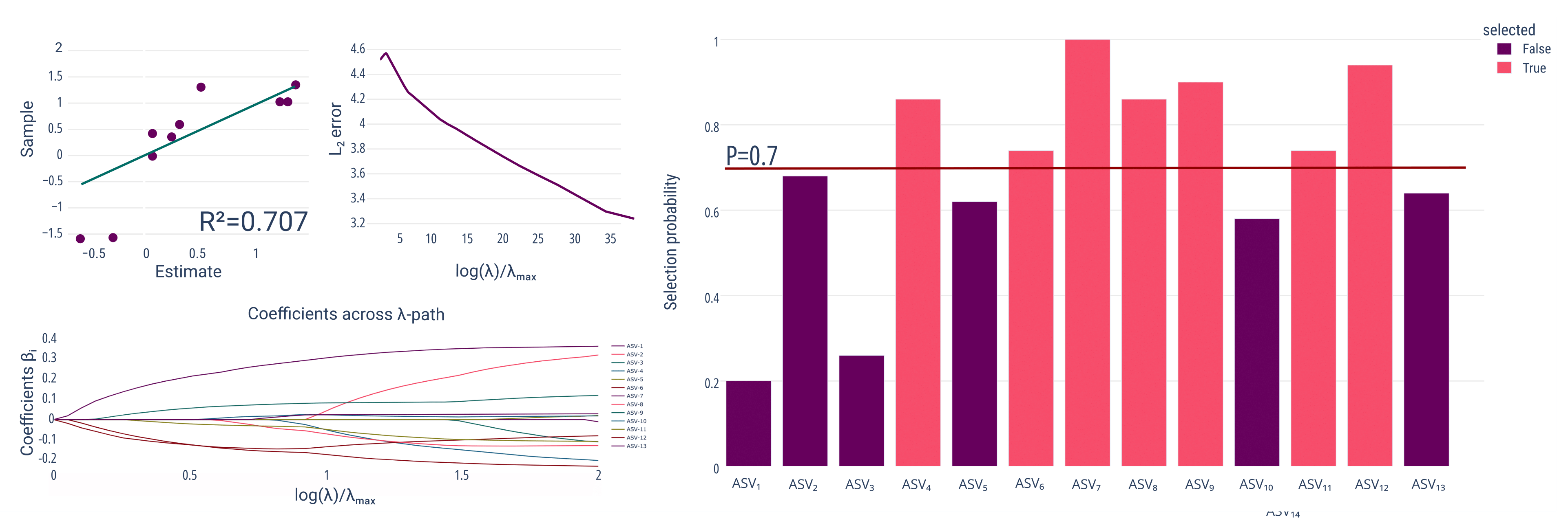
Fig. 11 The four panels a classo summarize regression report gives you, on the 13-ASV toy data. Top left: predicted against observed soil temperature on held-out samples. Top right: cross-validated \(L_2\) error along the \(\lambda\) path. Bottom left: every coefficient \(\beta_i\) as the penalty relaxes — the order in which taxa enter is the order of their apparent importance. Right: stability selection, the proportion of subsamples in which each ASV was selected, against a threshold.

Four questions, one panel each.

Does the model predict anything? The scatter, not the \(R^2\) alone. With \(R^2 = 0.707\) on 10 held-out samples, one influential point moves that number a lot — look at whether the cloud follows the line or whether two extremes are carrying it.

Was the penalty chosen sensibly? Look for a visible minimum in the CV curve. Here it descends and flattens rather than turning up, so the cross-validation does not strongly identify a best \(\lambda\). The --p-cv-one-se rule exists for exactly this situation, and this run disabled it (--p-no-cv-one-se).

Which taxa carry the signal? The coefficient paths. Taxa whose \(\beta\) leaves zero early and stays large contribute consistently along the path. Taxa that wander near zero do not. Because the coefficients must sum to zero, they come in opposing groups — a positive \(\beta\) is only meaningful relative to the negative ones.

Would those taxa be selected again? Stability selection resamples the data and counts how often each feature survives [M4]. Trust this panel when the coefficient path looks ambiguous. The threshold is a choice you make, not a result.

Note

The figure comes from a run at a stability threshold of 0.7, while the command above uses --p-stabsel-threshold 0.5. Expect more features above your line than above the one drawn here. The figure also carries a stray ASV₁₄ tick label — the toy table has 13 features, not 14.

Outputs

data/regresstaxa_lc.qza holds the fitted problem — the coefficient path, the CV curve and the stability-selection frequencies. Beside it sit the predictions on the held-out split and a .qzv rendering all four panels above.

The comparison worth making next is Tree-Aggregated Regression: the same outcome, the same samples, but predictors aggregated up the taxonomy. If a clade predicts better than its member ASVs, that is evidence the signal is phylogenetically coherent rather than carried by one organism.