Choosing the penalties

The 300-ASV Dataset ends with a correlation matrix over 300 features estimated from 54 samples. The sample covariance in that regime is singular and every network you could draw is, in some sense, consistent with the data, so the penalties decide the model rather than the data alone.

\(\lambda_1\) controls how many edges survive. \(\mu_1\) controls how much of the covariance is explained away by unobserved factors instead of by edges between ASVs.

Selecting \(\lambda_1\)

The extended Bayesian Information Criterion (eBIC) scores each candidate network by fit minus a penalty for the edges it spends; take the \(\lambda_1\) that scores lowest. The extra parameter \(\gamma\) sets how harshly extra edges are charged. This analysis uses \(\gamma = 0.3\), between Foygel and Drton’s conventional \(0.5\) and the toy-table default of \(0.01\).

qiime gglasso solve-problem \
    --i-covariance-matrix atacama-top-300-correlation.qza \
    --p-n-samples 54 \
    --p-no-latent \
    --p-path-scale linear \
    --p-lambda1-min 0.30 --p-lambda1-max 1.00 --p-n-lambda1 15 \
    --p-gamma 0.3 \
    --o-solution atacama-top-300-sgl-linear-path.qza

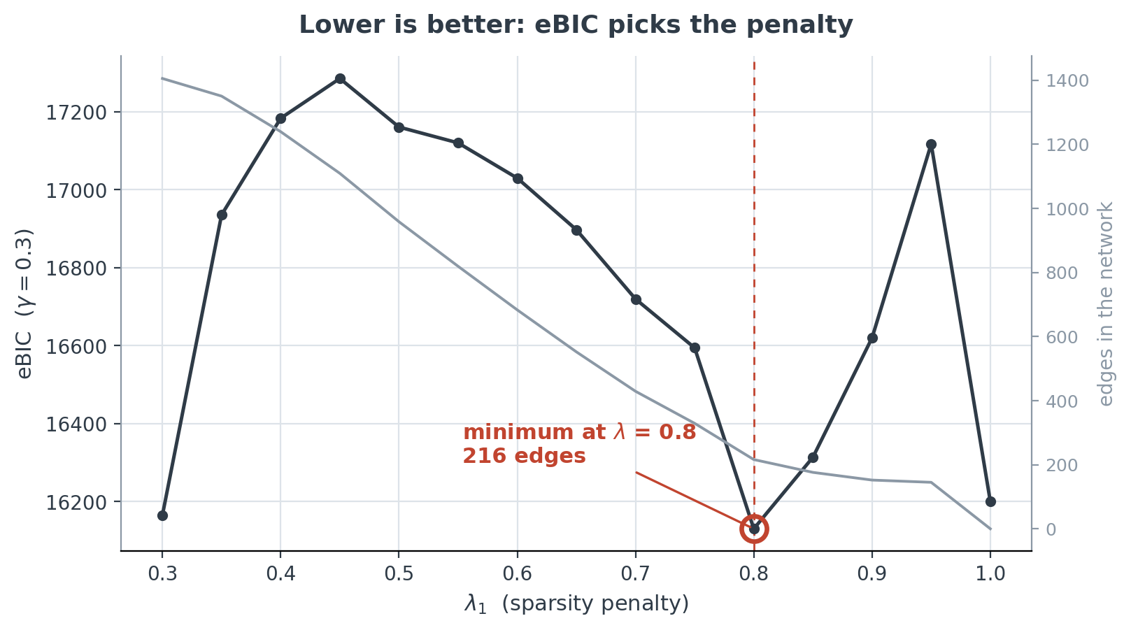
Fig. 16 eBIC across the linear \(\lambda_1\) path at \(\gamma = 0.3\), with the edge count on the right-hand axis. The minimum sits at \(\lambda_1 = 0.8\), giving a network of 216 edges among 300 ASVs — about 0.5% of the 44,850 possible pairs.

The minimum is real but shallow. eBIC at \(\lambda_1 = 0.8\) is 16130.1, and at the opposite end of the path \(\lambda_1 = 0.3\) scores 16165.1 — a difference of 35 on a scale of ~16,000. Two networks that differ by an order of magnitude in density (216 edges versus 1405) are nearly tied by this criterion. Do not quote the selected model as though the data had insisted on it.

The shallowness is why the answer moves with \(\gamma\): \(\gamma \in [0.30, 0.31]\) gives \(\lambda = 0.8\), \(\gamma \le 0.29\) gives the dense \(\lambda = 0.3\), and \(\gamma \ge 0.32\) gives the empty \(\lambda = 1.0\). The selection is a judgement about how much sparsity you want, expressed through \(\gamma\).

How we actually chose γ = 0.3

\(\gamma = 0.5\) is the conventional default and here selects the empty network. \(\gamma = 0.01\) — the plugin’s default, tuned for the 13-ASV toy table — selects 1405 edges, which at \(n = 54\) is far more parameters than data. We took the middle: the smallest \(\gamma\) that yields a network sparse enough to read. It sits very close to a boundary of the interval above, so we report the sensitivity rather than hide it.

The full path, generated by analysis/slurm/01_lambda_path.sh and rendered straight from docs/_data/atacama-lambda-path.tsv so that it cannot drift from the figure above:

Table 1 eBIC and edge count at every grid point

lambda	eBIC (gamma=0.3)	edges
1	16200.00	0
0.95	17117.10	145
0.9	16619.90	152
0.85	16313.58	176
0.8	16130.10	216
0.75	16594.22	329
0.7	16719.57	429
0.65	16897.21	552
0.6	17029.69	683
0.55	17120.00	819
0.5	17160.63	958
0.45	17285.22	1109
0.4	17183.28	1239
0.35	16935.41	1350
0.3	16165.13	1405

The per-\(\gamma\) comparison that produced the interval is in analysis/reports/.

Sizing the latent block

An edge between two ASVs is supposed to mean the two associate after controlling for everything else measured. Soil pH, moisture and depth act on many taxa at once, and a driver left out of the model deposits spurious edges among the taxa it drives.

The sparse + low-rank formulation gives those edges somewhere else to go: it splits the precision matrix into a sparse part \(\hat{\Theta}_S\) (the network) and a low-rank part \(\hat{L}\) (a handful of latent factors). The penalty \(\mu_1\) controls the rank — larger \(\mu_1\) permits fewer latent factors.

# rank 2 (mu1 = 15); repeat with mu1 = 10 for rank 5, mu1 = 7.5 for rank 10
qiime gglasso solve-problem \
    --i-covariance-matrix atacama-top-300-correlation.qza \
    --p-n-samples 54 \
    --p-latent \
    --p-lambda1-min 0.8 --p-lambda1-max 0.8 --p-n-lambda1 1 \
    --p-lambda2-min 0.1 --p-lambda2-max 0.1 --p-n-lambda2 1 \
    --p-mu1-min 15 --p-mu1-max 15 --p-n-mu1 1 \
    --o-solution atacama-top-300-slr-lambda0.8-rank2.qza

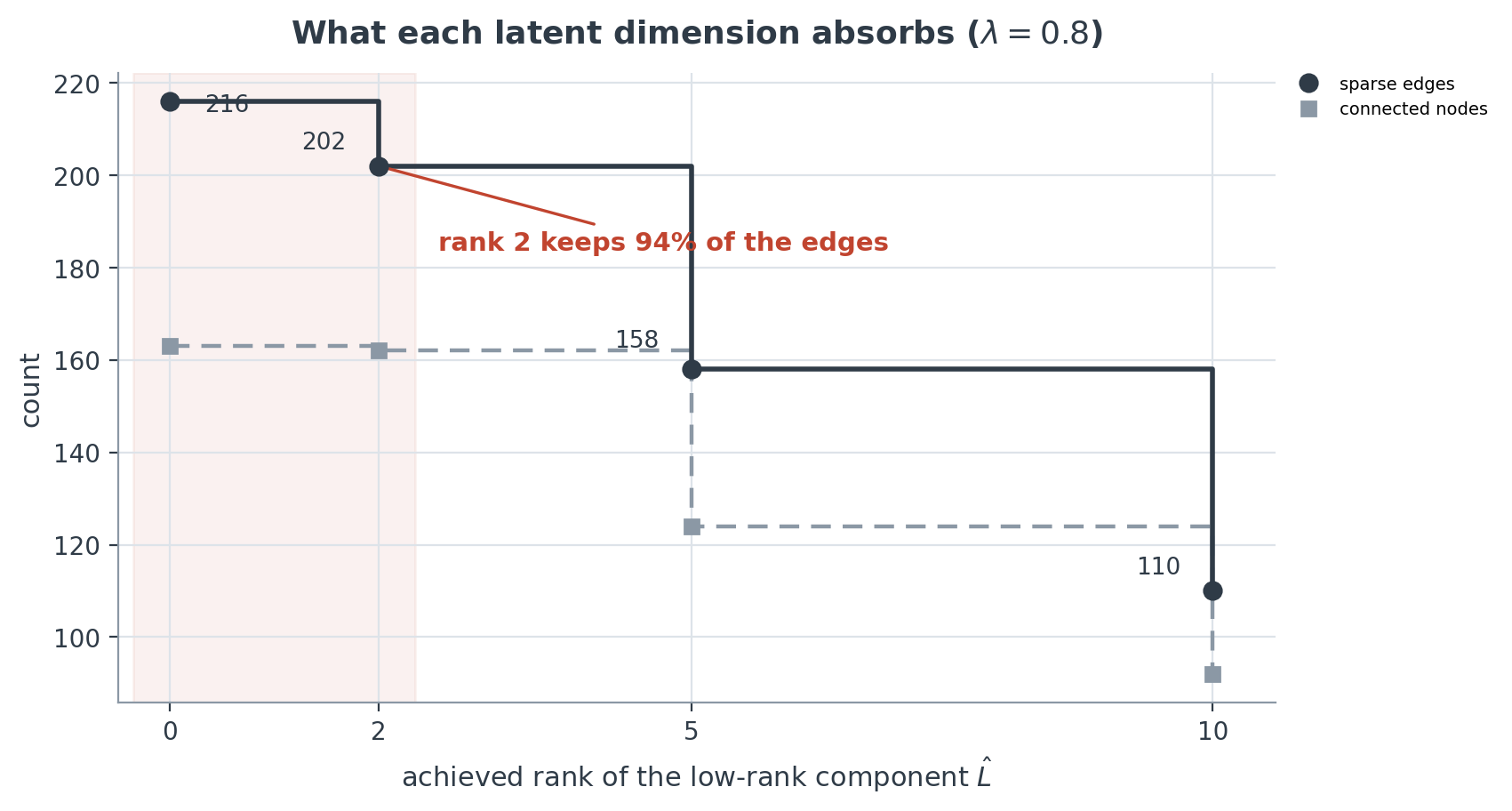
Fig. 17 Edges and connected nodes removed by each latent dimension. Two latent factors take 14 edges out of the network and cost one connected node; rank 10 removes half the edges and a third of the nodes. The rank is an output rather than a setting: it is reached by tuning \(\mu_1\), and these are the values that hit ranks 2, 5 and 10.

Rank 2 is the parsimonious choice. Its two latent components already capture the dominant measured-covariate structure: the network keeps 202 of its 216 edges and 162 of 163 connected nodes, so almost nothing that survived the sparsity penalty is explained away. Ranks 5 and 10 strip out progressively more, and at rank 10 you are no longer looking at the same network.

Independently, the strength of each downstream prediction task’s association with the robust principal components tracks the energy of its log-contrast coefficients in the rank-2 latent subspace (Spearman \(\rho = 0.90\), \(p = 6\times10^{-5}\)): two latent dimensions are enough to carry the signal the log-contrast models later need.

Setting the rank when you cannot set the rank

--p-rank is registered but currently guarded, pending upstream GGLasso support, so the rank is reached indirectly: fit at a few \(\mu_1\) values, read the achieved rank(lowrank_) from each solution, and keep the one that hits your target. For this dataset that is \(\mu_1 = 15, 10, 7.5\) for ranks \(2, 5, 10\).

The --p-lambda2-* triple pins the second penalty to a single value. The second penalty is inert for a single-graph problem, but leave the triple out and the solver puts lambda2 on a five-point default path, which turns this single fit into a model-selection run — see Choosing the Latent Rank.

Outputs

Two artifacts carry the result forward:

artifact	what it is
atacama-top-300-sgl-linear-path.qza	the whole \(\lambda\) path, with eBIC at every grid point
atacama-top-300-slr-lambda0.8-rank2.qza	the selected model: \(\lambda_1 = 0.8\), rank 2

The principal result is 216 edges at \(\lambda_1 = 0.8\), reduced to 202 once two latent factors are allowed. Choosing the Latent Rank examines the \(\mu_1 \to\) rank relationship in detail, and Latent PCA asks what the two latent axes are.