Network Interpretation and Analysis

The three estimators q2-gglasso implements — Single Graphical Lasso (SGL), Sparse + Low-Rank (SLR) and the Adaptive Graphical Lasso — return different networks from the same soil data. What separates them is what each is allowed to attribute an apparent correlation to: a direct edge, a latent factor, or a measured covariate.

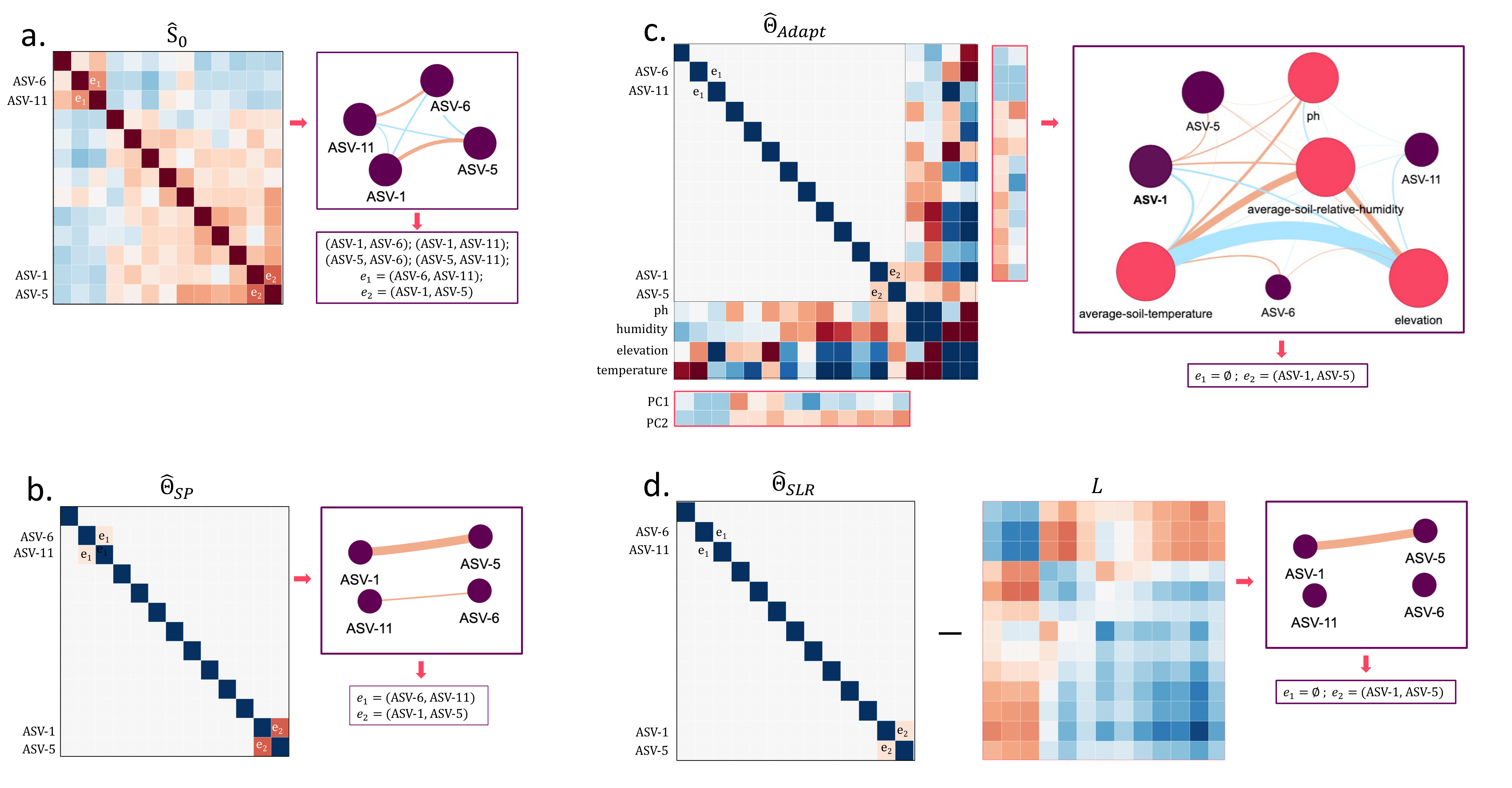
Fig. 9 The three estimators on the same 13-ASV data, at a fixed \(\lambda_1\). (a) the empirical covariance \(\hat{S}_0\) and the six relationships visible in it. (b) the sparse-only solution \(\hat{\Theta}_{SP}\) keeps two: \(e_1 = (\text{ASV-6}, \text{ASV-11})\) and \(e_2 = (\text{ASV-1}, \text{ASV-5})\). (d) at the same penalty, the sparse + low-rank solution keeps only \(e_2\) — the low-rank block \(L\) absorbs \(e_1\). (c) the adaptive solution, fit on a different covariance that includes the environmental covariates as nodes.

Important

The comparison holds \(\lambda_1\) fixed. Panels (b) and (d) share a penalty, so the single edge that disappears is attributable to the latent block. That is the only comparison in which “SLR gives fewer edges” means anything.

Do not read it as “SLR always yields a sparser network”. When each model picks its own penalty by eBIC, the counts can go the other way — on this same dataset SGL selects \(\lambda_1 = 0.4292\) and keeps 2 edges while SLR selects \(\lambda_1 = 0.2442\) and keeps 4. Adding latent variables gives the measurement and why the two comparisons answer different questions.

Panel (c) is not comparable to (b) or (d): it is fit on atacama-table-corr-meta.qza, which appends the covariates as additional variables, so its node set differs — see Adaptive Graphical Lasso.

Note

Reading taxon labels. transform-features keeps the original feature identifiers (see --p-keep-original-id), so network nodes and heatmap axes carry the ASV’s real ID and a selected feature traces directly back to its taxonomy. In the high-dimensional 300-ASV analysis, for example, the first taxon selected by the log-contrast models is a Pseudarthrobacter ASV — a genus emblematic of the Atacama soil biota, known for desiccation- and oligotrophy-tolerant lifestyles, pigment production, and survival in deep, hyperarid subsurface soils [D1, D4, D5].

Findings

• Environmental mediation. Elevation, pH, soil humidity and temperature mediate some of the apparent correlations between taxa.

• Direct interactions. Genuine microbial associations remain significant after you control for the environmental variables.

• Latent structure. The low-rank component carries systematic variation that may come from unmeasured factors or from global environmental gradients.

Reading the three fits together

• Compare SGL against SLR to distinguish direct from latent-mediated associations.

• Use the adaptive results to identify environment-independent microbial interactions.

• Check edge weights and stability across λ values before reporting an association.

Choosing a method

Method	Use when	What it gives you
SGL	Exploratory analysis No environmental data Complete association set Speed matters	Fast, complete network view
SLR	Suspected confounders Separate direct from indirect effects Batch effects present Focus on core interactions	Isolates direct associations
Adaptive model	Environmental data available Prior knowledge exists Focus on environment-independent edges Hypothesis-driven analysis	Uses prior knowledge, controls confounders

Moving on to q2-classo

With a network in hand, use q2-classo for regression and classification:

1. Feature selection. Use the identified microbial associations as candidate features for environmental or phenotype prediction.

2. Regression analysis. Model continuous outcomes with sparse microbial predictors.

3. Classification tasks. Predict a binary outcome from the selected microbial features.

4. Model selection. Validate predictive performance with classo’s built-in model selection methods.