Shotgun Metagenomics: mOTUs Profiles

The preceding chapters analyse 16S amplicon data from soil. The same two plugins apply to shotgun metagenomes from human infants, profiled to species level with mOTUs [S5].

The workflow is unchanged. transform-features, calculate-covariance, solve-problem, add-taxa and regress take the same arguments and carry the same meaning. The differences are the feature definition and the depth per feature: a feature here is a marker-gene-defined species rather than an exact sequence variant, and each count rests on far fewer reads. The lower depth determines which parameter values yield a usable model.

Study and data source

Qiita study	13241
ENA project	PRJEB52147
Publication	Bai-Tong et al., Scientific Reports 2022 [D6]
Design	preterm infants in two San Diego neonatal intensive care units, 9 whose mothers have asthma and 9 whose mothers do not

The MAP study (Microbiome, Atopic disease, and Prematurity) investigated whether maternal asthma is associated with differences in the preterm infant gut microbiome, metabolome, or both. The authors reported metabolomic differences between the two groups and concluded that maternal asthma “did not play an observable role in shaping the infant gut microbiome during the study period”. The bearing of this conclusion on the classification analysis is given under Limitations.

Note

Anonymous access requires a different URL from the one search engines return. qiita.ucsd.edu/study/description/13241 redirects to the Qiita landing page for unauthenticated visitors, which resembles a permissions error. The public view is qiita.ucsd.edu/public/?study_id=13241, and the endpoints under qiita.ucsd.edu/public_download/ require no account.

Data selection

The study contains two sequencing preparations covering the same samples: 16S V4 amplicon on an Illumina MiSeq, and whole-genome shotgun on a NovaSeq. Only the shotgun preparation is suitable for mOTUs profiling. PRJEB52147 comprises 192 runs, of which half are amplicon.

Within the shotgun preparation, analysis was restricted to faecal samples. The study also sequenced breast milk and meconium; these represent distinct microbial niches, and pooling them would confound a single covariance estimate with sample type. The restriction yields 36 runs from 18 infants, each contributing one early sample (10–18 days) and one late sample (23–47 days).

Preprocessing

Profiling requires 13 GiB of sequencing reads and the 2.9 GiB mOTUs reference database. The corresponding pipeline stages are analysis/slurm/32–35 in the repository accompanying this book; the steps are given here in summary.

1. Run selection. The Qiita sample template is joined to the ENA run report on the stripped sample_alias field, retaining records with library_strategy == WGS and sample_type == feces.

2. Retrieval and verification. 72 FASTQ files, each checked against the MD5 digest published by ENA.

3. Profiling. qiime motus profile is applied per sample and the results merged. mOTUs counts only reads aligning to ten universal marker genes, so a 2 M-read run yields on the order of several hundred assigned inserts.

4. Removal of the unassigned feature. mOTUs emits an explicit unassigned row for reads it cannot place. This row is the complement of the profiled fraction, and retaining it in a log-ratio transform would define the composition over a mixture of taxa and non-taxa.

5. Filtering. Two samples fall below 100 assigned counts and are excluded, leaving 34. Features present in fewer than two of the remaining samples are then dropped (378 → 156), and the 156 are ranked by total abundance with the 100 most abundant retained.

Important

Rank features by abundance, not by prevalence.

The table before filtering is 93.6% zeros (84.6% at a prevalence-3 floor). Two features absent from the same 28 samples exhibit a large sample correlation attributable entirely to shared zeros. A prevalence filter retains such a pair provided each feature clears the threshold; an abundance filter excludes them, because a feature whose entire signal consists of a small number of single counts contributes negligible total abundance.

The two filters select different models. Under prevalence filtering, the extended BIC selects the empty graph at every threshold examined. Under abundance filtering it selects a network exceeding a permutation null by three orders of magnitude. The data and the commands are identical in both cases.

Dataset characteristics

Table 4 Properties of the filtered table

property	value
samples (n)	34
features (p)	100
p/n	2.9
zeros	85.4%
median assigned depth	814
infants	18
samples per infant	16×2 + 2×1
diagnosis balance	17 asthma / 17 control

With \(p = 100\) and \(n = 34\) the sample covariance has rank at most 33 and is therefore singular. In this regime the penalty determines the model.

Two properties distinguish this table from the Atacama data:

• Sparsity. 85% of entries are zero, compared with a dense soil table. This motivates the mclr transform in place of clr.

• Repeated measures. Sixteen infants contribute two samples and two contribute one, the second having been dropped at the depth threshold. The covariance estimate is unaffected. The cross-validated regression is affected; see Limitations.

Obtaining the files

Three artifacts are distributed with this book:

BASE=https://raw.githubusercontent.com/Vlasovets/q2-hdstats-docs/main/docs/_data/motus
curl -L -O "${BASE}/motus-top100-table.qza"      # 20 KB, FeatureTable[Frequency]
curl -L -O "${BASE}/motus-top100-taxonomy.qza"   # 16 KB, FeatureData[Taxonomy]
curl -L -O "${BASE}/motus-outcomes.tsv"          # 1 KB, sample metadata

Network inference with q2-gglasso

Transformation and covariance estimation

qiime gglasso transform-features \
    --i-table motus-top100-table.qza \
    --i-taxonomy motus-top100-taxonomy.qza \
    --p-transformation mclr \
    --p-keep-original-id \
    --o-transformed-table mclr.qza

qiime gglasso calculate-covariance \
    --i-table mclr.qza \
    --p-method scaled \
    --o-covariance-matrix correlation.qza

Saved FeatureTable[Frequency] to: mclr.qza
Saved PairwiseFeatureData to: correlation.qza

--i-taxonomy is a required input of transform-features although the function body does not read it. Pass the taxonomy you will need for add-taxa rather than a placeholder.

Selection of \(\lambda_1\)

qiime gglasso solve-problem \
    --i-covariance-matrix correlation.qza \
    --p-n-samples 34 \
    --p-no-latent \
    --p-path-scale linear \
    --p-lambda1-min 0.05 --p-lambda1-max 1.0 --p-n-lambda1 20 \
    --p-gamma 0.15 \
    --o-solution motus-sgl-path.qza

Saved GGLassoProblem to: motus-sgl-path.qza

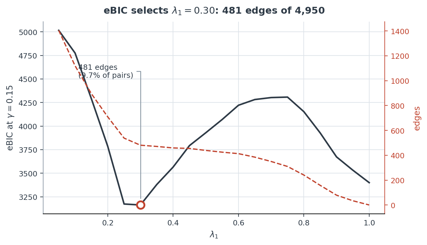
Fig. 22 Extended BIC along the \(\lambda_1\) path at \(\gamma = 0.15\) (solid, left axis) with the corresponding edge count (dashed, right axis). The minimum is interior, both adjacent grid points scoring higher, and occurs at \(\lambda_1 = 0.30\). The selected model contains 481 edges among 4,950 possible pairs, a density of 9.7%.

The value \(\gamma = 0.15\) differs from the \(\gamma = 0.3\) used for the Atacama data. At \(\gamma \geq 0.20\) the criterion selects the empty graph on this dataset, the model-space penalty dominating the likelihood term at \(n = 34\). Report \(\gamma\) with any network you derive from it.

qiime gglasso summarize \
    --i-solution motus-sgl-path.qza \
    --p-label-size 6pt \
    --o-visualization motus-sgl-summary.qzv

Saved Visualization to: motus-sgl-summary.qzv

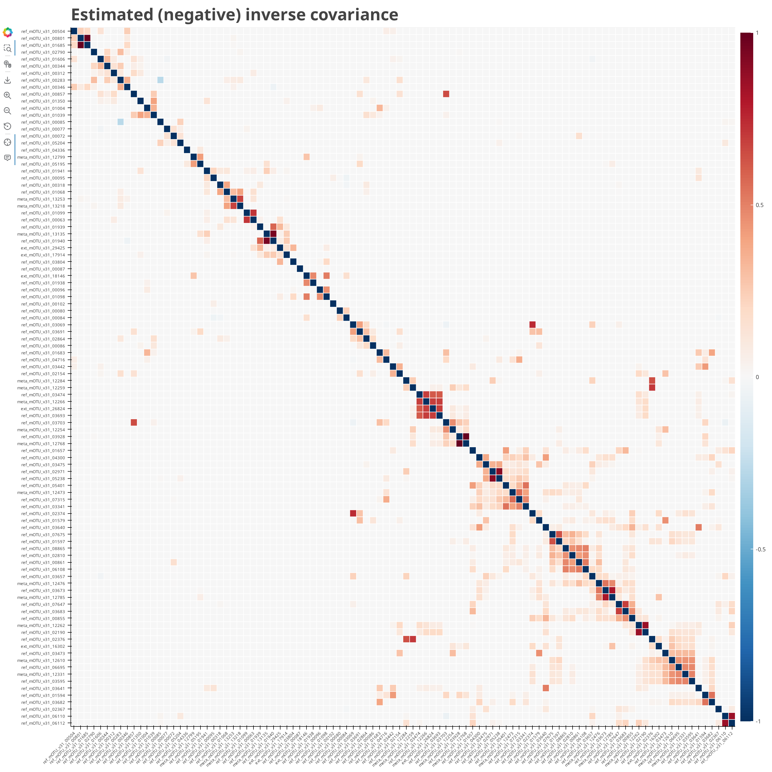
Fig. 23 The Estimated inverse covariance tab of motus-sgl-summary.qzv, at the selected \(\lambda_1 = 0.30\). The off-diagonal entries are the 481 retained edges; the remaining 90.3% of the 4,950 pairs are exactly zero. The Statistics tab of the same visualization reports best lambda 0.3 and a sparsity of 0.0972, which is \(481 / 4{,}950\).

Download: motus-sgl-summary.qzv — solution path, sparsity and extended BIC at each grid point. View at view.qiime2.org.

Sparse plus low-rank decomposition

qiime gglasso solve-problem \
    --i-covariance-matrix correlation.qza \
    --p-n-samples 34 \
    --p-latent \
    --p-lambda1-min 0.30 --p-lambda1-max 0.30 --p-n-lambda1 1 \
    --p-lambda2-min 0.1 --p-lambda2-max 0.1 --p-n-lambda2 1 \
    --p-mu1-min 5 --p-mu1-max 5 --p-n-mu1 1 \
    --o-solution motus-slr-mu5.qza

Saved GGLassoProblem to: motus-slr-mu5.qza

All three penalties are pinned to single values. Leave --p-lambda2-* unset and the solver substitutes a five-point default path, which turns the single fit into a model-selection run that may select a \(\lambda_1\) other than the one specified.

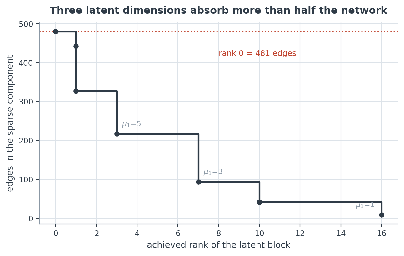
Fig. 24 Achieved rank against the number of edges retained in the sparse component. The rank is an output rather than a setting: --p-rank is registered but raises an exception on all released versions of GGLasso, so a target rank is reached by tuning \(\mu_1\) and reading back the achieved value. At \(\mu_1 = 5\) the rank is 3 and 217 of the 481 edges remain.

Three latent dimensions remove 264 of the 481 edges (55%). The corresponding figure for the Atacama data is 6.5%, where a rank-2 block removes 14 of 216 edges. In the Atacama analysis the latent block removes few edges (Choosing the Latent Rank). That interpretation does not transfer to this dataset.

The eigenvalues of the latent block at \(\mu_1 = 5\) are 2.428, 0.711 and 0.029. The third is small relative to the first two, so the fit is close to rank 2 with a weak third direction.

qiime gglasso pca \
    --i-solution motus-slr-mu5.qza \
    --i-table mclr.qza \
    --m-sample-metadata-file motus-outcomes.tsv \
    --p-n-components 3 \
    --o-visualization motus-latent-pca.qzv

Saved Visualization to: motus-latent-pca.qzv

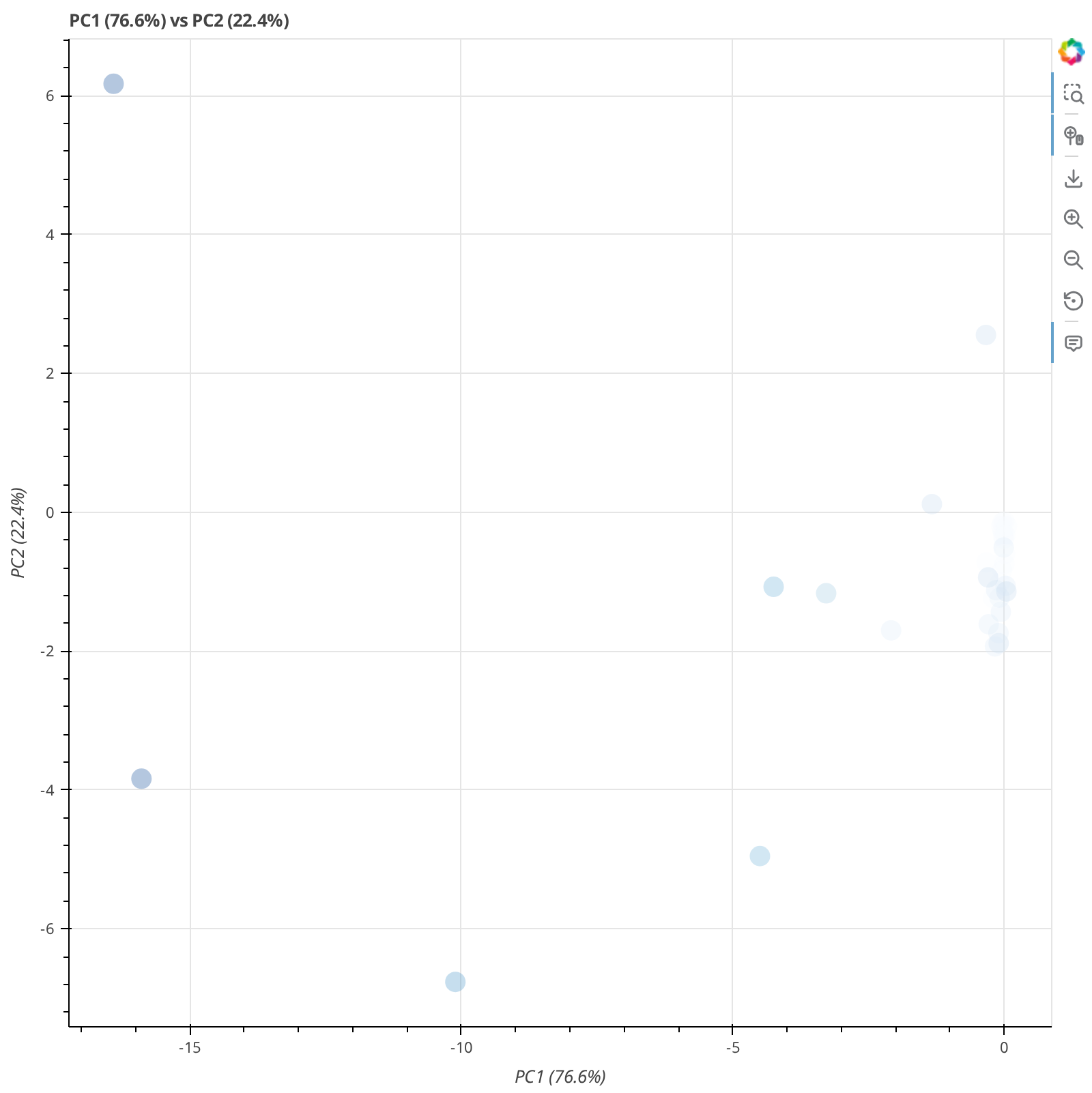
Fig. 25 The Single plot tab of motus-latent-pca.qzv: samples projected onto the first two latent components. The two components carry 76.6% and 22.4% of the latent variance, 99.0% together, which is the rank-2-plus-weak-third structure the eigenvalues describe. Most samples fall near the origin of PC1 with a small number displaced along it.

Download: motus-latent-pca.qzv — samples projected onto the latent components, coloured by metadata.

--p-n-components must not exceed the achieved rank. The action also requires --m-sample-metadata-file, despite the signature marking it optional.

Log-contrast regression with q2-classo

The response variable is host_age_days, postnatal age at sampling, ranging from 10 to 47 days.

It is the only numeric variable in this metadata that varies within an infant. Gestational age at birth, birth weight and maternal age are constant per infant, so 34 samples would carry no more information than 18 for those responses. Postnatal age varies by 13 to 29 days within each infant.

qiime classo transform-features \
    --i-features motus-top100-table.qza \
    --o-x classo-x.qza

qiime classo add-taxa \
    --i-features classo-x.qza \
    --i-taxa motus-top100-taxonomy.qza \
    --o-x classo-x-trac.qza \
    --o-aweights classo-w-trac.qza

Saved FeatureTable[Design] to: classo-x.qza
Saved FeatureTable[Design] to: classo-x-trac.qza
Saved Weights to: classo-w-trac.qza

add-taxa reconstructs the design as \(\log(X)A\), where \(A\) aggregates features along the taxonomy, so that coefficients are associated with clades rather than individual species. The design grows from 100 columns to 133, the additional 33 corresponding to internal taxonomic nodes.

This requires distinct leaf labels, which not all taxonomies provide. The mOTUs lineage terminates in m__<mOTU_id>, so all 100 leaves are distinct even where two mOTUs share a species name. A taxonomy containing duplicate leaves merges the corresponding features into a single node.

qiime classo regress \
    --i-features classo-x-trac.qza \
    --i-weights classo-w-trac.qza \
    --m-y-file motus-outcomes.tsv \
    --m-y-column host_age_days \
    --p-concomitant \
    --p-path --p-path-nlam-log 60 --p-path-lamin-log 0.001 \
    --p-cv --p-cv-subsets 5 --p-cv-seed 1 --p-no-cv-one-se \
    --p-cv-nlam 60 --p-cv-lamin 0.001 --p-cv-logscale \
    --p-no-stabsel --p-no-lamfixed \
    --o-result motus-regress-age.qza

Explanation:

• --p-concomitant estimates the noise scale jointly with the coefficients, so the penalty does not have to be calibrated against an assumed residual variance.

• --p-path and --p-cv are two independent grids. The path is for display; the cross-validation grid is what selects the model. Both are set to 60 points down to \(10^{-3}\lambda_{\max}\) here so that the two agree.

• --p-no-cv-one-se selects the cross-validated minimum rather than the sparsest model within one standard error of it. On this dataset the two differ; see below.

• --p-no-stabsel and --p-no-lamfixed suppress two further selection procedures that would otherwise run and lengthen the fit.

Saved CLASSOProblem to: motus-regress-age.qza

The cross-validated refit retains two of the 133 candidate clades:

clade	coefficient
o__Enterobacterales	+5.2475
p__Bacteroidetes	−5.2475

Enterobacterales increases and Bacteroidetes decreases with postnatal age over the 10–47 day window sampled here. The two coefficients are exact negatives and sum to zero to machine precision, which is the zero-sum constraint of the log-contrast formulation: the model is a single balance between two clades, and only their ratio is identified. The fitted intercept is +21.7318; postnatal age has mean 25.8 and median 20.5 days over these 34 samples.

Warning

Read coefficient labels from the artifact, never by position. c-lasso prepends the intercept to the coefficient vector, so the 133-column design yields 134 coefficients. A label list taken from the design columns is then shifted by one against them, and every selected clade is reported as its predecessor in the column order. The coefficient labels are stored beside the coefficients in the artifact and are also exported as CV-beta.csv inside the .qzv.

qiime classo summarize \
    --i-problem motus-regress-age.qza \
    --p-maxplot 40 \
    --o-visualization motus-regress-summary.qzv

Saved Visualization to: motus-regress-summary.qzv

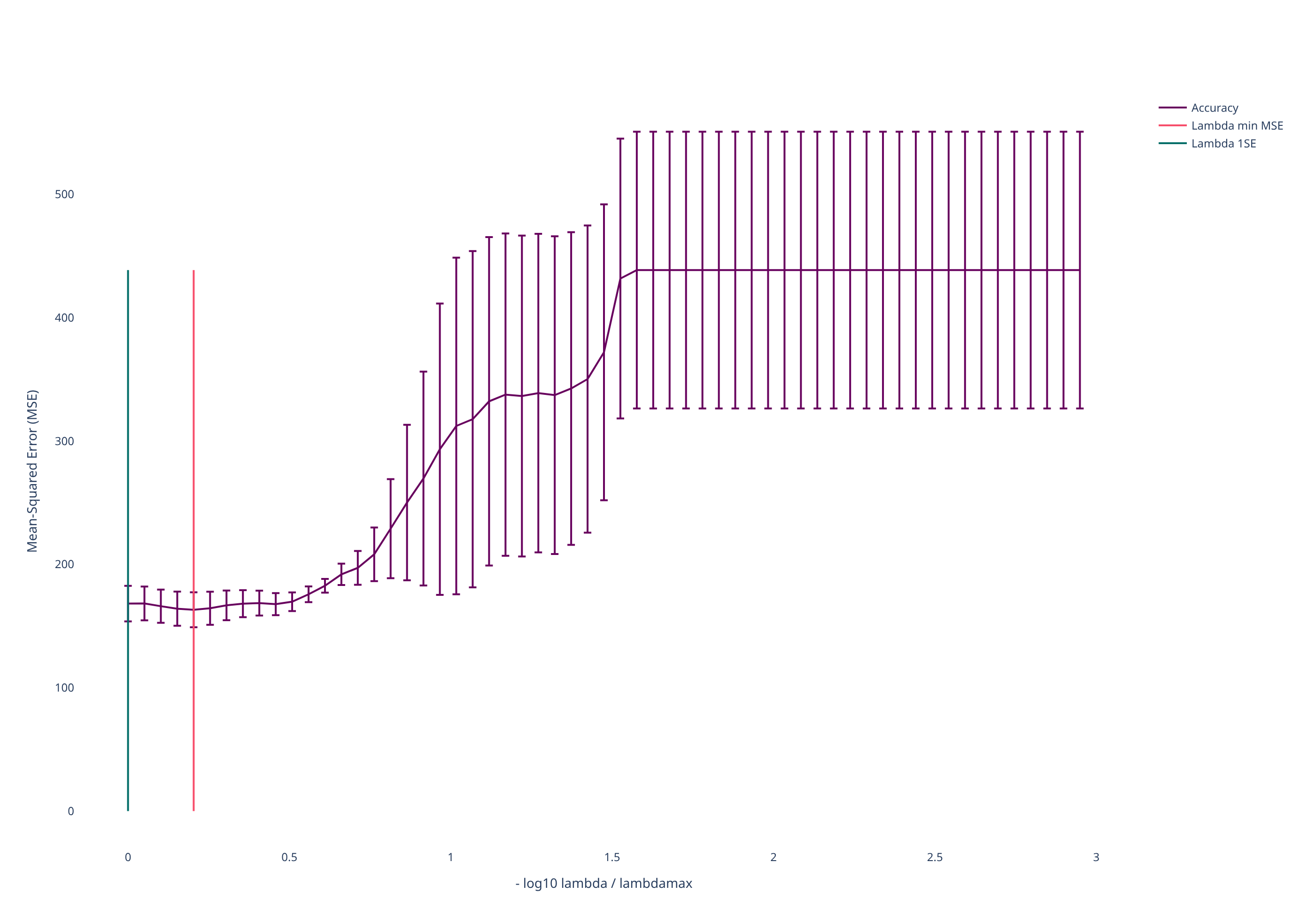
Fig. 26 The cross-validation curve from motus-regress-summary.qzv. The horizontal axis is \(-\log_{10}(\lambda / \lambda_{\max})\), so the left edge is the maximal penalty and the right edge the minimal one. Mean-squared error is 168.2 at \(\lambda_{\max}\), falls to a minimum of 163.2, and rises to 438.6 as the penalty is removed and the model overfits. The two vertical lines mark the cross-validated minimum and the one-standard-error choice.

--p-no-cv-one-se is material to this result. The one-standard-error rule returns the sparsest model within one standard error of the cross-validated minimum. Here the minimum is 163.2 with a standard error of 14.1, so the rule admits any model scoring below 177.3 — and the intercept-only model, at 168.2, qualifies. The one-standard-error line in Fig. 26 therefore sits at \(\lambda_{\max}\), where no coefficient is active. Both rules read the same cross-validation curve; they differ only in which point on it they take.

Note

The selected model improves on the intercept-only model by 5.0 mean-squared-error units, which is 0.35 standard errors. The two clades are the best that cross-validation can find, but the curve does not establish that they beat predicting the mean.

Download: motus-regress-summary.qzv — the \(\lambda\) path, cross-validation curve and selected coefficients. --p-maxplot applies to the aggregated design, which is wider than the input table.

Limitations and interpretation

Network density. 481 edges represent 9.7% of all pairs, against 0.48% for the 300-ASV Atacama network. Estimating 481 edges from 34 samples is over-parameterised irrespective of the selection criterion. Evidence that the estimate reflects structure rather than noise comes from a permutation null: re-solving five times with each feature column permuted independently across samples — removing all between-feature dependence while preserving each marginal distribution, including its zeros — yields a mean of 0.2 edges and a maximum of 1.

Cross-validation leakage. Sixteen infants contribute two samples each, and --p-cv-subsets partitions at random with no grouping option, so one sample of a pair may fall in the training set and the other in the test set. Holding out whole infants instead gives:

response	metric	baseline	subject holdout	sample holdout	difference
host_age_days	\(R^2\)	0.0	+0.164	−0.041	−0.205
diagnosis	accuracy	0.500	0.471	0.588	+0.118

The differences have opposite signs. diagnosis is a property of the infant, so a paired sample discloses the label and the random partition inflates the estimate. Postnatal age varies within an infant, so a paired sample discloses nothing about it and the leaky estimate is merely noisier. The direction of the bias therefore depends on whether the response is constant within a subject.

Important

q2-classo exposes --p-cv-subsets and --p-cv-seed but no grouping parameter. The subject-held-out figures above were obtained by calling the classo API directly (analysis/slurm/42_subject_holdout.sh). For designs with repeated measures the plugin’s cross-validation does not implement the required partition. State this in any methods description that relies on it.

The classification result is negative. Held out by infant, prediction of maternal asthma from the microbiome achieves 0.471 accuracy against a majority-class baseline of 0.500. With 9 subjects per group a 95% confidence interval on any accuracy estimate spans approximately ±0.23, so this does not demonstrate the absence of an effect; it is consistent with the conclusion reported by [D6] from a more complete analysis.

Sample size is the limiting factor. Eighteen infants, rather than the choice of profiler or filter, is what requires \(\gamma\) to be reduced to 0.15, produces a network of this density, and bounds the achievable \(R^2\).

Outputs

artifact	contents
motus-sgl-path.qza	the \(\lambda_1\) path with extended BIC at 20 grid points
motus-slr-mu5.qza	the selected model, \(\lambda_1 = 0.30\) at rank 3
motus-regress-age.qza	the trac regression of postnatal age
three .qzv files	linked above

The principal results are 481 edges at \(\lambda_1 = 0.30\), reduced to 217 when three latent factors are admitted, and a two-clade balance associated with postnatal age at a subject-held-out \(R^2\) of +0.164.

Interpretation addresses the corresponding question for the Atacama data: whether the structure the network attributes to unobserved drivers is the structure the log-contrast model exploits.