

Log-Contrast Classification#
Log-Contrast Regression predicted a continuous outcome. The same community now faces a yes/no question: can you tell a vegetated site from a bare one by its microbes alone?
The compositional problem is unchanged — only ratios between features are meaningful — so the zero-sum constraint on the coefficients carries over. What changes is the loss: a hinge loss on a binary label instead of squared error, and a misclassification rate instead of \(R^2\).
Important
qiime classo classify has no --p-concomitant parameter. It is forced off
internally, and passing it fails. The regression action accepts it. The
classification action does not.
Step 1: Transform Features#
Apply CLR transformation to the count data:
qiime classo transform-features \
    --p-transformation clr \
    --p-coef 0.5 \
    --i-features data/atacama-counts.qza \
    --o-x data/xclr
Step 2: Add Covariates#
Include environmental metadata with custom weights:
qiime classo add-covariates \
    --i-features data/xclr.qza \
    --m-covariates-file data/atacama-selected-covariates-veg.tsv \
    --p-to-add ph average-soil-relative-humidity elevation average-soil-temperature vegetation \
    --p-w-to-add 1. 0.1 0.1 0.1 1 \
    --o-new-features data/xcovariates_lc \
    --o-new-c data/ccovariates_lc \
    --o-new-w data/wcovariates_lc
Step 3: Split Data#
Create training and test sets for classification analysis:
qiime sample-classifier split-table \
    --i-table data/xcovariates_lc.qza \
    --m-metadata-file data/atacama-selected-covariates-veg.tsv \
    --m-metadata-column vegetation \
    --p-test-size 0.2 \
    --p-random-state 42 \
    --p-stratify False \
    --o-training-table data/classify-xtraining_lc.qza \
    --o-test-table data/classify-xtest_lc.qza \
    --o-training-targets data/classify-training-targets_lc.qza \
    --o-test-targets data/classify-test-targets_lc.qza
Step 4: Train the Classification Model#
Train a log-contrast classifier using cross-validation to predict vegetation presence:
qiime classo classify \
    --i-features data/classify-xtraining_lc.qza \
    --i-c data/ccovariates_lc.qza \
    --i-weights data/wcovariates_lc.qza \
    --m-y-file data/atacama-selected-covariates-veg.tsv \
    --m-y-column vegetation \
    --p-huber False \
    --p-stabsel \
    --p-cv \
    --p-path \
    --p-lamfixed \
    --p-stabsel-threshold 0.5 \
    --p-cv-seed 42 \
    --p-no-cv-one-se \
    --o-result data/classifytaxa_lc.qza
Parameters explained:
--i-features: Training feature table--i-c: C matrix carrying the log-contrast constraints--i-weights: Feature weights--m-y-column vegetation: Target variable, vegetation presence or absence--p-huber False: Use standard logistic loss--p-stabsel: Run stability selection alongside the path fit--p-cv: Choose the penalty by cross-validation--p-stabsel-threshold 0.5: Stability selection threshold
Step 5: Make Predictions#
Apply the trained model to test data:
qiime classo predict \
    --i-features data/classify-xtest_lc.qza \
    --i-problem data/classifytaxa_lc.qza \
    --o-predictions data/classify-predictions_lc.qza
Step 6: Generate Summary Visualization#
Render the fitted classifier and its predictions as a report:
qiime classo summarize \
    --i-problem data/classifytaxa_lc.qza \
    --i-predictions data/classify-predictions_lc.qza \
    --o-visualization data/classifytaxa_C1_lc.qzv
Open it with qiime tools view or at QIIME 2 View.
Reading the result#
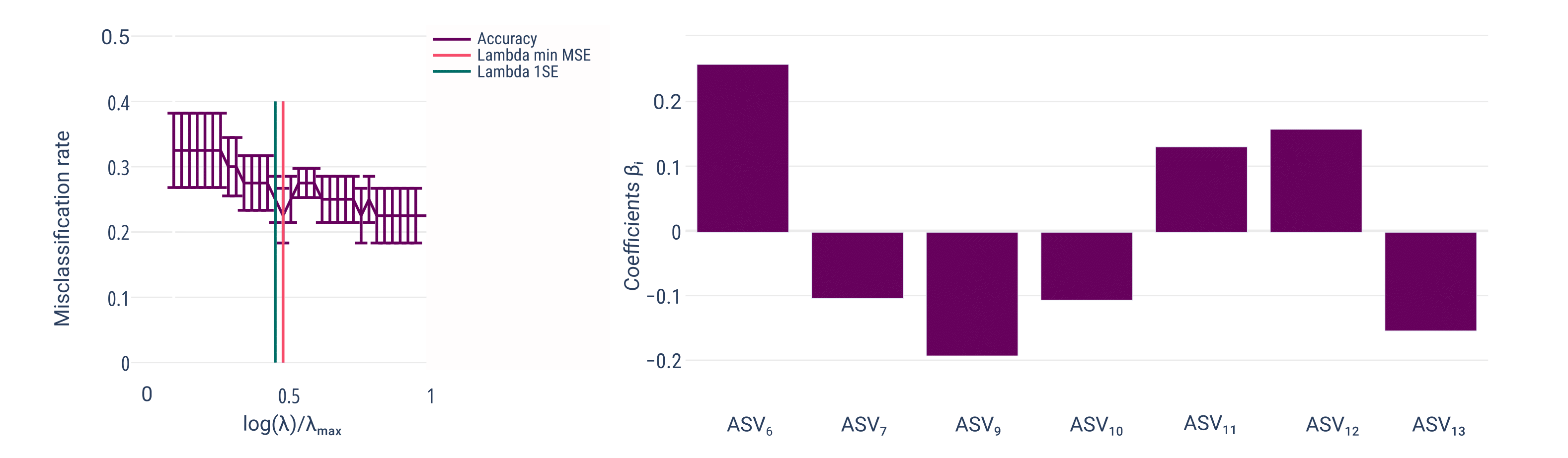
Fig. 13 Classification on the 13-ASV toy data. Left: cross-validated misclassification rate along the \(\lambda\) path, with error bars over folds and vertical lines at the minimum-error \(\lambda\) and at the more conservative one-standard-error choice. Right: the coefficients of the seven ASVs the selected model retains.#
The cross-validation is not confident here. The misclassification rate sits between roughly 0.22 and 0.33 across the whole path, and the error bars overlap almost everywhere. The two candidate penalties — the minimum and the one-standard-error rule — land on top of each other, which happens when the curve has no clear minimum to separate them. On 50 samples with a binary outcome, expect a curve like this one. The model distinguishes vegetated from bare sites better than a coin, and not much more.
Do not skip past that to the coefficient panel. A coefficient list from a model whose error curve is flat tells you which features the optimiser happened to keep at one point on a path where neighbouring points would have kept others. Model Selection covers what to do about it. Stability selection, as in the regression workflow, is the usual answer.
The coefficients come in opposing groups. Seven ASVs are retained, three with positive weight and four negative, and they sum to approximately zero — the log-contrast constraint, not a coincidence of the fit. No single coefficient can be read alone: ASV-6’s \(+0.26\) is a statement about ASV-6 relative to the negatively-weighted set, not about its abundance.
Note
The legend labels the plotted series “Accuracy” while the axis is labelled misclassification rate. The axis is correct: the values are error rates, so a lower curve is a better model. The legend is wrong.
Outputs#
data/classifytaxa_lc.qza holds the fitted classifier. Beside it sit the
predictions on the held-out split and a .qzv showing both panels above.
Before drawing conclusions from the selected taxa, read Model Interpretation. With an error curve this flat, the comparison in Tree-Aggregated Classification is the more informative next step: if aggregating to clades sharpens the CV curve, the signal is phylogenetic rather than ASV-specific.