High-Dimensional Example: q2-classo on 300 Atacama ASVs

This chapter applies q2-classo to the same 300-ASV, 54-sample Atacama design used in the high-dimensional graphical-lasso chapter, predicting each continuous environmental covariate from the microbiome with cross-validated log-contrast regression. It reproduces the reference analysis of Christian L. Müller.

Setup

Each of the 15 continuous covariates is used once as the outcome; missing outcome values are mean-imputed. Models use the standard log-contrast formulation R1 with an intercept, selected by 5-fold cross-validation with the one-standard-error rule along a log-spaced \(\lambda\) path:

qiime classo regress \
    --i-features atacama-top-300-clr-design.qza \
    --m-y-file atacama-classo-outcomes-mean-imputed.tsv \
    --m-y-column <outcome> \
    --p-do-yshift --p-path --p-path-nlam-log 100 --p-path-lamin-log 0.001 \
    --p-cv --p-cv-subsets 5 --p-cv-seed 1 --p-cv-one-se \
    --p-cv--nlam 100 --p-cv-lamin 0.001 --p-cv-logscale \
    --p-no-stabsel --p-no-lamfixed --p-no-concomitant --p-no-huber --p-intercept \
    --o-result <outcome>-r1-cv5.qza

Prediction from ASVs only (base R1)

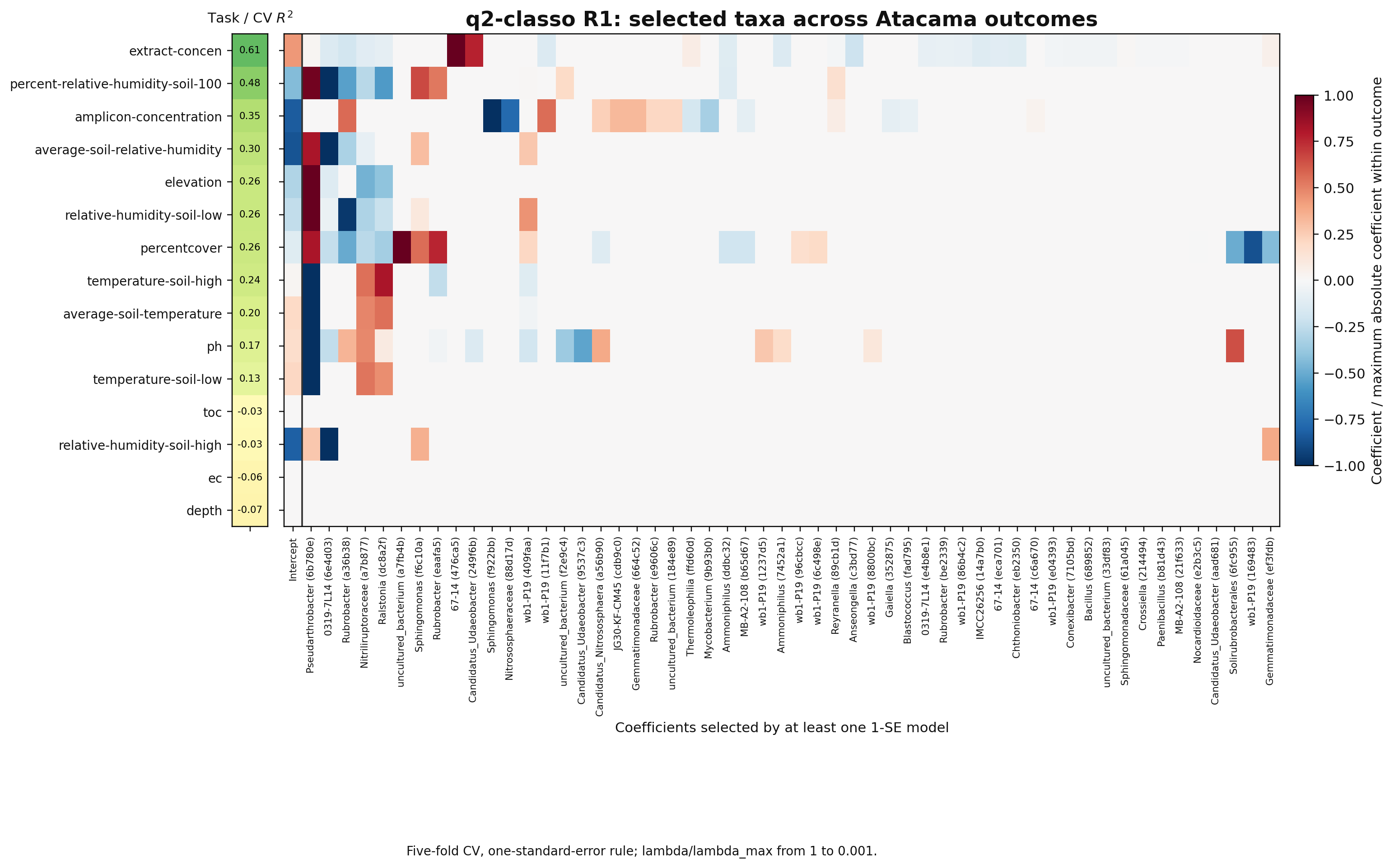
The out-of-sample \(R^2\) (mean across the 5 folds) shows which environmental variables are predictable from the 300 ASVs alone:

Outcome	CV \(R^2\)
extract-concen	0.61
percent-relative-humidity-soil-100	0.48
amplicon-concentration	0.35
average-soil-relative-humidity	0.30
elevation	0.26
relative-humidity-soil-low	0.26
percentcover	0.26
temperature-soil-high	0.24
average-soil-temperature	0.20
ph	0.17
temperature-soil-low	0.13
toc / relative-humidity-soil-high / ec / depth	\(\le 0\)

The first selected taxon (largest-magnitude coefficient column, after the intercept) is a Pseudarthrobacter ASV — a genus characteristic of the Atacama soil community (see the interpretation notes).

Adjusting for environmental covariates (joint and filtered)

Two variants add the other covariates as extra predictors (each rescaled and L2-normalized, covariate penalty weight 0.1626):

• Joint — add all other covariates as predictors.

• Filtered adjustment — add only covariates that are not strongly correlated with the outcome (Pearson \(\lvert r\rvert < 0.80\)), so a covariate that is essentially a proxy for the outcome cannot leak it.

This is a two-step workflow. First, build the augmented design by adding the chosen covariate(s) to the ASV design (this produces new features, constraint, and weights artifacts):

qiime classo add-covariates \
    --i-features atacama-top-300-clr-design.qza \
    --m-covariates-file atacama-classo-outcomes-mean-imputed.tsv \
    --p-to-add <covariate> --p-rescale --p-w-to-add 0.162565105 \
    --o-new-features <design>.qza --o-new-c <c>.qza --o-new-w <w>.qza

Then run the same cross-validated regression as before, but on the augmented design (passing the constraint and weights from the previous step):

qiime classo regress \
    --i-features <design>.qza --i-c <c>.qza --i-weights <w>.qza \
    --m-y-file atacama-classo-outcomes-mean-imputed.tsv --m-y-column <outcome> \
    --p-do-yshift --p-path --p-path-nlam-log 120 --p-path-lamin-log 0.0001 \
    --p-cv --p-cv-subsets 5 --p-cv-seed 1 --p-cv-one-se \
    --p-cv--nlam 120 --p-cv-lamin 0.0001 --p-cv-logscale \
    --p-no-stabsel --p-no-lamfixed --p-no-concomitant --p-no-huber --p-intercept \
    --o-result <outcome>-joint-r1-cv5.qza

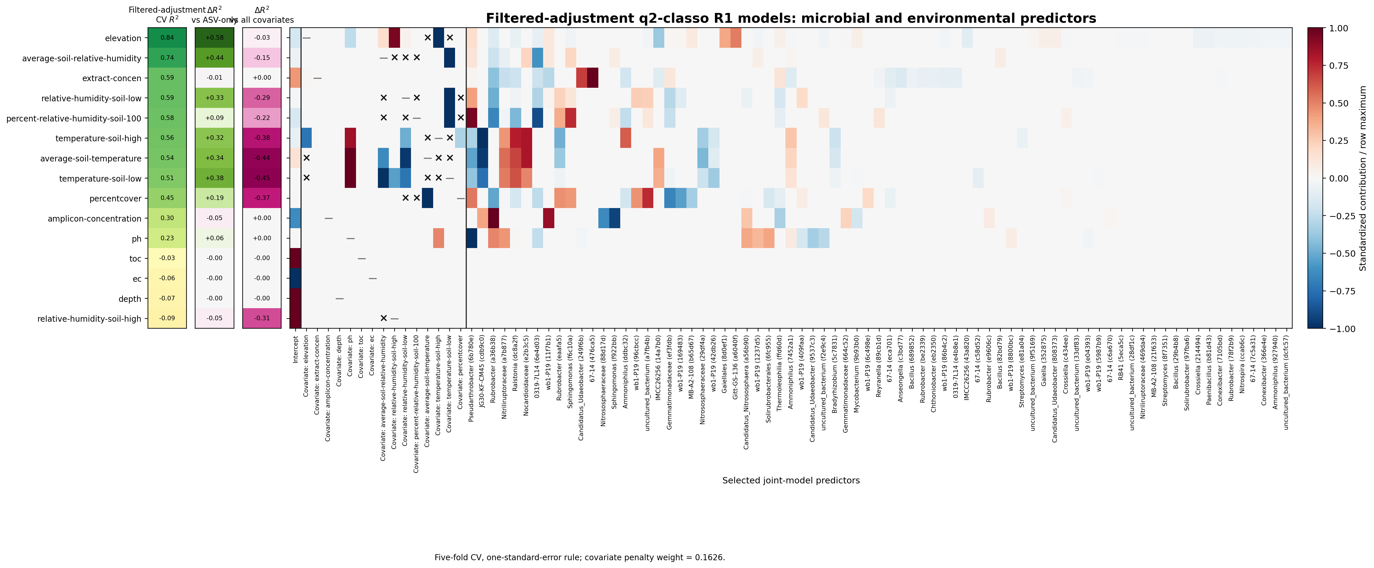
Adding covariates sharply increases predictability of the physically-coupled variables — e.g. soil temperature and humidity — but the filtered analysis removes most of that gain, showing it came largely from outcome-correlated covariates rather than the microbiome:

Outcome	ASV-only	Joint (all cov.)	Filtered (\(\lvert r\rvert<0.8\))
average-soil-temperature	0.20	0.98	0.54
temperature-soil-low	0.13	0.96	0.51
temperature-soil-high	0.24	0.94	0.56
average-soil-relative-humidity	0.30	0.88	0.74
relative-humidity-soil-low	0.26	0.88	0.59
elevation	0.26	0.87	0.84
percentcover	0.26	0.81	0.45
percent-relative-humidity-soil-100	0.48	0.80	0.58
extract-concen	0.61	0.59	0.59

Elevation stands out: its filtered \(R^2\) (0.84) stays close to the joint value (0.87), i.e. its predictability does not depend on outcome-correlated covariates. For the temperature variables, by contrast, the joint gain (≈ 0.94–0.98) collapses under filtering (≈ 0.51–0.56), a textbook illustration of why task-specific covariate filtering matters.